1 Linear Equations in Linear Algebra
1.1 Systems of Linear Equations
A 3x3 system having a unique solution is solved by putting the augmented matrix in reduced row echelon form. A picture of three intersecting planes provides geometric intuition.

Example of solving a 3-by-3 system of linear equations by row-reducing the augmented matrix, in the case of one solution math.la.e.linsys.3x3.soln.row_reduce.o
Definition of matrix in reduced row echelon form math.la.d.mat.rref
Linear systems have zero, one, or infinitely many solutions. math.la.t.linsys.zoi
Definition of consistent linear system math.la.d.linsys.consistent
- Created On
- February 15th, 2017
- 7 years ago
- Views
- 3
- Type
- Video
- Timeframe
- Review
- Perspective
- Example
- Language
- English
- Content Type
- text/html; charset=utf-8
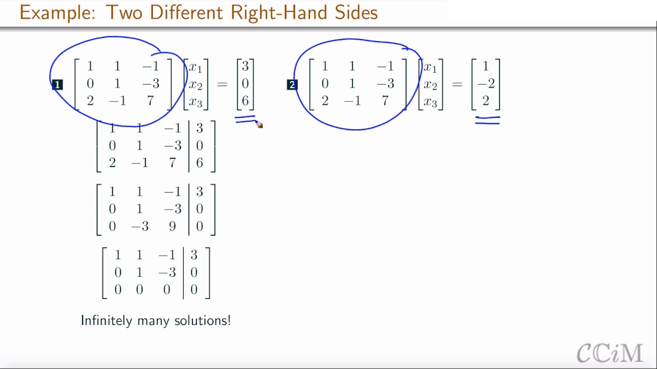
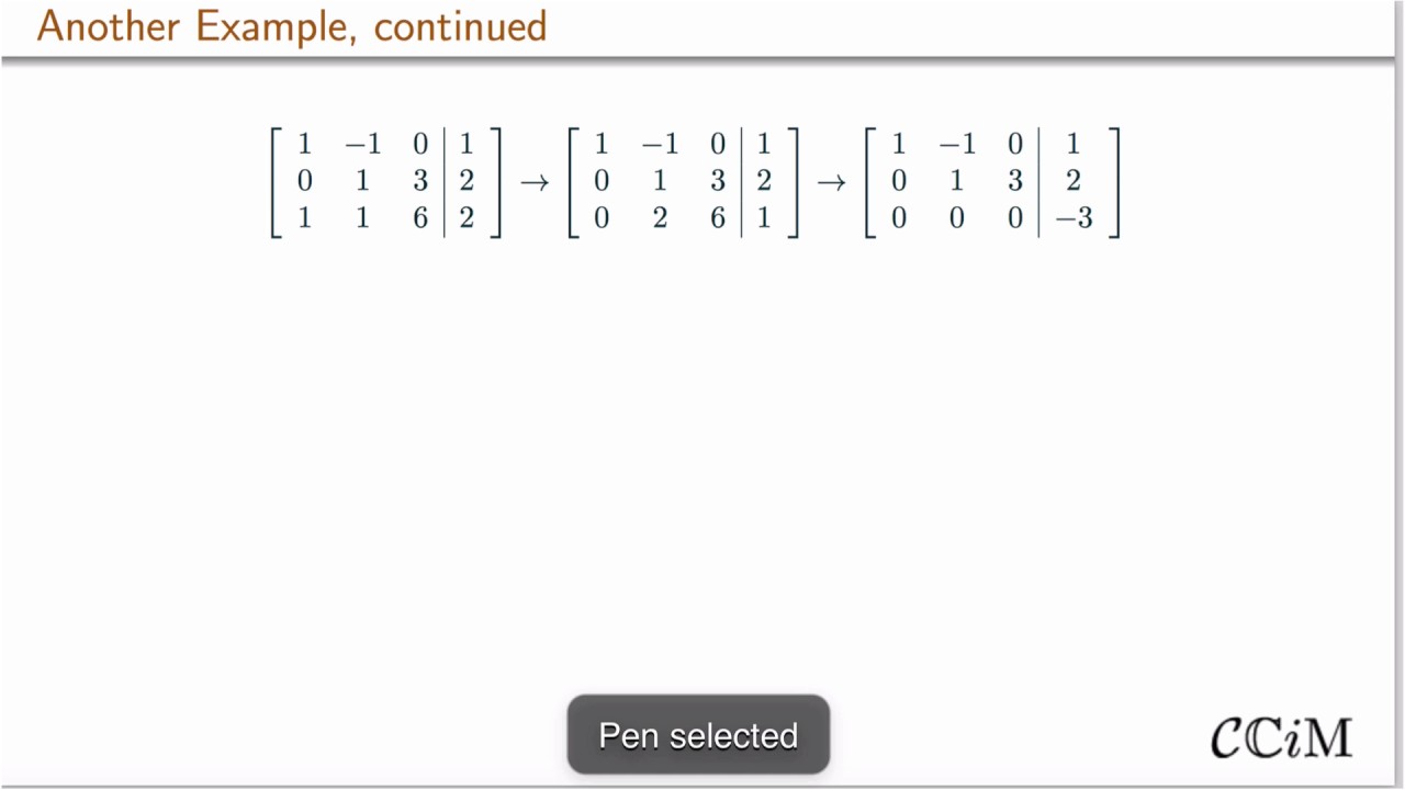
A 3x3 matrix equation Ax=b is solved for two different values of b. In one case there is no solution, and in another there are infinitely many solutions. These examples illustrate a theorem about linear combinations of the columns of the matrix A.
Example of solving a 3-by-3 system of linear equations by row-reducing the augmented matrix, in the case of no solutions math.la.e.linsys.3x3.soln.row_reduce.z
Example of solving a 3-by-3 system of linear equations by row-reducing the augmented matrix, in the case of infinitely many solutions math.la.e.linsys.3x3.soln.row_reduce.i
The matrix equation Ax=b has a solution if and only if b is a linear combination of the columns of A. math.la.t.mat.eqn.lincomb
Definition of matrix equation math.la.d.mat.eqn
- Created On
- February 15th, 2017
- 7 years ago
- Views
- 3
- Type
- Video
- Timeframe
- Pre-class
- Perspective
- Example
- Language
- English
- Content Type
- text/html; charset=utf-8
The reduced row echelon form is used to determine when a 3x3 system is inconsistent. A picture of planes in 3-dimensional space is used to provide geometric intuition.
Example of solving a 3-by-3 system of linear equations by row-reducing the augmented matrix, in the case of no solutions math.la.e.linsys.3x3.soln.row_reduce.z
- Created On
- February 15th, 2017
- 7 years ago
- Views
- 4
- Type
- Video
- Timeframe
- Review
- Perspective
- Example
- Language
- English
- Content Type
- text/html; charset=utf-8
Sample problems to help understand when a linear system has 0, 1, or infinitely many solutions.

Linear systems have zero, one, or infinitely many solutions. math.la.t.linsys.zoi
math.la.t.rref.consistent
- Created On
- February 15th, 2017
- 7 years ago
- Views
- 2
- Type
- Handout
- Timeframe
- In-class
- Perspective
- Example
- Language
- English
- Content Type
- text/html; charset=utf-8
Notation for matrix entries, diagonal matrix, square matrix, identity matrix, and zero matrix.

Notation for entry of matrix math.la.d.mat.entry
Definition of m by n matrix math.la.d.mat.m_by_n
Definition of diagonal matrix math.la.d.mat.diagonal
Definition of identity matrix math.la.d.mat.identity
Definition of zero matrix math.la.d.mat.zero
- Created On
- February 17th, 2017
- 7 years ago
- Views
- 3
- Type
- Video
- Timeframe
- Pre-class
- Perspective
- Introduction
- Language
- English
- Content Type
- text/html; charset=utf-8
Equivalence of systems of linear equations, row operations, corresponding matrices representing the linear systems

Definition of equivalent systems of linear equations math.la.d.linsys.equiv
Definition of row operations on a matrix math.la.d.mat.row_op
Definition of row equivalent matrices math.la.d.mat.row_equiv
Row equivalent matrices represent equivalent linear systems math.la.t.mat.row_equiv.linsys
Example of putting a matrix in echelon form math.la.e.mat.echelon.of
- Created On
- August 21st, 2017
- 7 years ago
- Views
- 2
- Type
- Video
- Language
- English
- Content Type
- text/html; charset=utf-8
How to compute all solutions to a general system $Ax=b$ of linear equations and connection to the corresponding homogeneous system $Ax=0$. Visualization of the geometry of solution sets. Consistent systems and their solution using row reduction.

Example of solving a 3-by-3 homogeneous system of linear equations by row-reducing the augmented matrix, in the case of infinitely many solutions math.la.e.linsys.3x3.soln.homog.row_reduce.i
Definition of homogeneous linear system of equations math.la.d.linsys.homog
A homogeneous system has a nontrivial solution if and only if it has a free variable. math.la.t.linsys.homog.nontrivial
Parametric vector form of the solution set of a system of linear equations math.la.c.linsys.soln_set.vec
Definition of trivial solution to a homogeneous linear system of equations math.la.d.linsys.homog.trivial
Definition of nontrivial solution to a homogeneous linear system of equations math.la.d.linsys.homog.nontrivial
- Created On
- August 22nd, 2017
- 7 years ago
- Views
- 3
- Type
- Video
- Language
- English
- Content Type
- text/html; charset=utf-8
Homogeneous systems of linear equations; trivial versus nontrivial solutions of homogeneous systems; how to find nontrivial solutions; how to know from the reduced row-echelon form of a matrix whether the corresponding homogeneous system has nontrivial solutions.

Definition of homogeneous linear system of equations math.la.d.linsys.homog
Definition of trivial solution to a homogeneous linear system of equations math.la.d.linsys.homog.trivial
Definition of nontrivial solution to a homogeneous linear system of equations math.la.d.linsys.homog.nontrivial
A homogeneous system has a nontrivial solution if and only if it has a free variable. math.la.t.linsys.homog.nontrivial
Example of solving a 3-by-3 homogeneous system of linear equations by row-reducing the augmented matrix, in the case of infinitely many solutions math.la.e.linsys.3x3.soln.homog.row_reduce.i
- Created On
- August 25th, 2017
- 7 years ago
- Views
- 4
- Type
- Video
- Language
- English
- Content Type
- text/html; charset=utf-8
We will motivate our study of linear algebra by considering the problem of solving several linear equations simultaneously. The word solve tends to get abused somewhat, as in “solve this problem.” When talking about equations we understand a more precise meaning: find all of the values of some variable quantities that make an equation, or several equations, simultaneously true.
Definition of system of linear equations math.la.d.linsys
- License
- GFDL-1.2
- Submitted At
- September 11th, 2017
- 7 years ago
- Views
- 3
- Type
- Textbook
- Language
- English
- Content Type
- text/html
We will motivate our study of linear algebra by considering the problem of solving several linear equations simultaneously. The word solve tends to get abused somewhat, as in “solve this problem.” When talking about equations we understand a more precise meaning: find all of the values of some variable quantities that make an equation, or several equations, simultaneously true.
Definition of solution set of a system of linear equations math.la.d.linsys.soln_set
- License
- GFDL-1.2
- Submitted At
- September 11th, 2017
- 7 years ago
- Views
- 2
- Type
- Textbook
- Language
- English
- Content Type
- text/html
We begin our study of linear algebra with an introduction and a motivational example.
Definition of linear equation math.la.d.lineqn
- License
- GFDL-1.2
- Submitted At
- September 11th, 2017
- 7 years ago
- Views
- 2
- Type
- Textbook
- Language
- English
- Content Type
- text/html
We will motivate our study of linear algebra by considering the problem of solving several linear equations simultaneously. The word solve tends to get abused somewhat, as in “solve this problem.” When talking about equations we understand a more precise meaning: find all of the values of some variable quantities that make an equation, or several equations, simultaneously true.
Definition of solution to a system of linear equations math.la.d.linsys.soln
- License
- GFDL-1.2
- Submitted At
- September 11th, 2017
- 7 years ago
- Views
- 2
- Type
- Textbook
- Language
- English
- Content Type
- text/html
We will motivate our study of linear algebra by considering the problem of solving several linear equations simultaneously. The word solve tends to get abused somewhat, as in “solve this problem.” When talking about equations we understand a more precise meaning: find all of the values of some variable quantities that make an equation, or several equations, simultaneously true.
Definition of equivalent systems of linear equations math.la.d.linsys.equiv
- License
- GFDL-1.2
- Submitted At
- September 11th, 2017
- 7 years ago
- Views
- 3
- Type
- Textbook
- Language
- English
- Content Type
- text/html
After solving a few systems of equations, you will recognize that it does not matter so much what we call our variables, as opposed to what numbers act as their coefficients. A system in the variables \(x_1,\,x_2,\,x_3\) would behave the same if we changed the names of the variables to \(a,\,b,\,c\) and kept all the constants the same and in the same places. In this section, we will isolate the key bits of information about a system of equations into something called a matrix, and then use this matrix to systematically solve the equations. Along the way we will obtain one of our most important and useful computational tools.
Definition of matrix math.la.d.mat
Definition of m by n matrix math.la.d.mat.m_by_n
math.la.c.mat.entry
- License
- GFDL-1.2
- Submitted At
- September 11th, 2017
- 7 years ago
- Views
- 3
- Type
- Textbook
- Language
- English
- Content Type
- text/html
After solving a few systems of equations, you will recognize that it does not matter so much what we call our variables, as opposed to what numbers act as their coefficients. A system in the variables \(x_1,\,x_2,\,x_3\) would behave the same if we changed the names of the variables to \(a,\,b,\,c\) and kept all the constants the same and in the same places. In this section, we will isolate the key bits of information about a system of equations into something called a matrix, and then use this matrix to systematically solve the equations. Along the way we will obtain one of our most important and useful computational tools.
Definition of row operations on a matrix math.la.d.mat.row_op
- License
- GFDL-1.2
- Submitted At
- September 11th, 2017
- 7 years ago
- Views
- 2
- Type
- Textbook
- Language
- English
- Content Type
- text/html
After solving a few systems of equations, you will recognize that it does not matter so much what we call our variables, as opposed to what numbers act as their coefficients. A system in the variables \(x_1,\,x_2,\,x_3\) would behave the same if we changed the names of the variables to \(a,\,b,\,c\) and kept all the constants the same and in the same places. In this section, we will isolate the key bits of information about a system of equations into something called a matrix, and then use this matrix to systematically solve the equations. Along the way we will obtain one of our most important and useful computational tools.
Definition of coefficient matrix of a linear system math.la.d.mat.coeff
- License
- GFDL-1.2
- Submitted At
- September 11th, 2017
- 7 years ago
- Views
- 3
- Type
- Textbook
- Language
- English
- Content Type
- text/html
After solving a few systems of equations, you will recognize that it does not matter so much what we call our variables, as opposed to what numbers act as their coefficients. A system in the variables \(x_1,\,x_2,\,x_3\) would behave the same if we changed the names of the variables to \(a,\,b,\,c\) and kept all the constants the same and in the same places. In this section, we will isolate the key bits of information about a system of equations into something called a matrix, and then use this matrix to systematically solve the equations. Along the way we will obtain one of our most important and useful computational tools.
Definition of augmented matrix of a linear system math.la.d.mat.augmented
- License
- GFDL-1.2
- Submitted At
- September 11th, 2017
- 7 years ago
- Views
- 3
- Type
- Textbook
- Language
- English
- Content Type
- text/html
After solving a few systems of equations, you will recognize that it does not matter so much what we call our variables, as opposed to what numbers act as their coefficients. A system in the variables \(x_1,\,x_2,\,x_3\) would behave the same if we changed the names of the variables to \(a,\,b,\,c\) and kept all the constants the same and in the same places. In this section, we will isolate the key bits of information about a system of equations into something called a matrix, and then use this matrix to systematically solve the equations. Along the way we will obtain one of our most important and useful computational tools.
Definition of row equivalent matrices math.la.d.mat.row_equiv
- License
- GFDL-1.2
- Submitted At
- September 11th, 2017
- 7 years ago
- Views
- 2
- Type
- Textbook
- Language
- English
- Content Type
- text/html
We will now be more careful about analyzing the reduced row-echelon form derived from the augmented matrix of a system of linear equations. In particular, we will see how to systematically handle the situation when we have infinitely many solutions to a system, and we will prove that every system of linear equations has either zero, one or infinitely many solutions. With these tools, we will be able to routinely solve any linear system.
Linear systems have zero, one, or infinitely many solutions. math.la.t.linsys.zoi
- License
- GFDL-1.2
- Submitted At
- September 11th, 2017
- 7 years ago
- Views
- 3
- Type
- Textbook
- Language
- English
- Content Type
- text/html
We will now be more careful about analyzing the reduced row-echelon form derived from the augmented matrix of a system of linear equations. In particular, we will see how to systematically handle the situation when we have infinitely many solutions to a system, and we will prove that every system of linear equations has either zero, one or infinitely many solutions. With these tools, we will be able to routinely solve any linear system.
Definition of consistent linear system math.la.d.linsys.consistent
Definition of inconsistent linear system math.la.d.linsys.inconsistent
- License
- GFDL-1.2
- Submitted At
- September 11th, 2017
- 7 years ago
- Views
- 3
- Type
- Textbook
- Language
- English
- Content Type
- text/html
After solving a few systems of equations, you will recognize that it does not matter so much what we call our variables, as opposed to what numbers act as their coefficients. A system in the variables \(x_1,\,x_2,\,x_3\) would behave the same if we changed the names of the variables to \(a,\,b,\,c\) and kept all the constants the same and in the same places. In this section, we will isolate the key bits of information about a system of equations into something called a matrix, and then use this matrix to systematically solve the equations. Along the way we will obtain one of our most important and useful computational tools.
Row equivalent matrices represent equivalent linear systems math.la.t.mat.row_equiv.linsys
- License
- GFDL-1.2
- Submitted At
- September 11th, 2017
- 7 years ago
- Views
- 3
- Type
- Textbook
- Language
- English
- Content Type
- text/html
Definition of coefficients of a linear equation math.la.d.lineqn.coeff
Definition of size of a matrix math.la.d.mat.size
Example of solving a 3-by-3 homogeneous system of linear equations by row-reducing the augmented matrix, in the case of one solution math.la.e.linsys.3x3.soln.homog.row_reduce.o
1.2 Row Reduction and Echelon Forms
A 3x3 system having a unique solution is solved by putting the augmented matrix in reduced row echelon form. A picture of three intersecting planes provides geometric intuition.
Example of solving a 3-by-3 system of linear equations by row-reducing the augmented matrix, in the case of one solution math.la.e.linsys.3x3.soln.row_reduce.o
Definition of matrix in reduced row echelon form math.la.d.mat.rref
Linear systems have zero, one, or infinitely many solutions. math.la.t.linsys.zoi
Definition of consistent linear system math.la.d.linsys.consistent
- Created On
- February 15th, 2017
- 7 years ago
- Views
- 3
- Type
- Video
- Timeframe
- Review
- Perspective
- Example
- Language
- English
- Content Type
- text/html; charset=utf-8
Equivalence of systems of linear equations, row operations, corresponding matrices representing the linear systems
Definition of equivalent systems of linear equations math.la.d.linsys.equiv
Definition of row operations on a matrix math.la.d.mat.row_op
Definition of row equivalent matrices math.la.d.mat.row_equiv
Row equivalent matrices represent equivalent linear systems math.la.t.mat.row_equiv.linsys
Example of putting a matrix in echelon form math.la.e.mat.echelon.of
- Created On
- August 21st, 2017
- 7 years ago
- Views
- 2
- Type
- Video
- Language
- English
- Content Type
- text/html; charset=utf-8
Definition of echelon form, reduction of a matrix to echelon form in order to compute solutions to systems of linear equations; definition of reduced row echelon form

Definition of (row) echelon form of a matrix math.la.d.mat.echelon.of
Example of (echelon matrix/matrix in (row) echelon form) math.la.e.mat.echelon
Definition of matrix in reduced row echelon form math.la.d.mat.rref
Definition of reduced row echelon form of a matrix math.la.d.mat.rref.of
Definition of leading entry in a row of a matrix math.la.d.mat.row.leading
Definition of (echelon matrix/matrix in (row) echelon form) math.la.d.mat.echelon
Example of putting a matrix in echelon form math.la.e.mat.echelon.of
- Created On
- August 25th, 2017
- 7 years ago
- Views
- 2
- Type
- Video
- Language
- English
- Content Type
- text/html; charset=utf-8
After solving a few systems of equations, you will recognize that it does not matter so much what we call our variables, as opposed to what numbers act as their coefficients. A system in the variables \(x_1,\,x_2,\,x_3\) would behave the same if we changed the names of the variables to \(a,\,b,\,c\) and kept all the constants the same and in the same places. In this section, we will isolate the key bits of information about a system of equations into something called a matrix, and then use this matrix to systematically solve the equations. Along the way we will obtain one of our most important and useful computational tools.
Every matrix is row-equivalent to a matrix in reduced row echelon form. math.la.t.mat.rref.exists
- License
- GFDL-1.2
- Submitted At
- September 11th, 2017
- 7 years ago
- Views
- 3
- Type
- Textbook
- Language
- English
- Content Type
- text/html
After solving a few systems of equations, you will recognize that it does not matter so much what we call our variables, as opposed to what numbers act as their coefficients. A system in the variables \(x_1,\,x_2,\,x_3\) would behave the same if we changed the names of the variables to \(a,\,b,\,c\) and kept all the constants the same and in the same places. In this section, we will isolate the key bits of information about a system of equations into something called a matrix, and then use this matrix to systematically solve the equations. Along the way we will obtain one of our most important and useful computational tools.
Every matrix is row-equivalent to only one matrix in reduced row echelon form. math.la.t.mat.rref.unique
- License
- GFDL-1.2
- Submitted At
- September 11th, 2017
- 7 years ago
- Views
- 2
- Type
- Textbook
- Language
- English
- Content Type
- text/html
After solving a few systems of equations, you will recognize that it does not matter so much what we call our variables, as opposed to what numbers act as their coefficients. A system in the variables \(x_1,\,x_2,\,x_3\) would behave the same if we changed the names of the variables to \(a,\,b,\,c\) and kept all the constants the same and in the same places. In this section, we will isolate the key bits of information about a system of equations into something called a matrix, and then use this matrix to systematically solve the equations. Along the way we will obtain one of our most important and useful computational tools.
Definition of matrix in reduced row echelon form math.la.d.mat.rref
Definition of pivot column math.la.d.mat.pivot_col
Definition of leading entry in a row of a matrix math.la.d.mat.row.leading
- License
- GFDL-1.2
- Submitted At
- September 11th, 2017
- 7 years ago
- Views
- 3
- Type
- Textbook
- Language
- English
- Content Type
- text/html
Definition of row reduce a matrix math.la.d.mat.row_reduce
Definition of pivot position math.la.d.mat.pivot_position
Example of putting a matrix in echelon form and identifying the pivot columns math.la.e.mat.echelon.of.pivot
math.la.e.mat.echelon.of.4x4
Definition of pivot math.la.d.mat.pivot
math.la.d.insys.variable.basic
math.la.d.insys.variable.free
math.la.e.linsys.3x5.soln.row_reduce.i
The echelon form can be used to determine if a linear system is consistent. math.la.t.echelon.consistent
Example of using the echelon form to determine if a linear system is consistent. math.la.e.echelon.consistent
1.3 Vector Equations
The product of a matrix times a vector is defined, and used to show that a system of linear equations is equivalent to a system of linear equations involving matrices and vectors. The example uses a 2x3 system.

Definition of matrix-scalar multiplication math.la.d.mat.scalar.mult
A linear system is equivalent to a vector equation. math.la.t.linsys.vec
A matrix equation is equivalent to a linear system math.la.t.mat.eqn.linsys
- License
- CC-BY-SA-4.0
- Created On
- February 15th, 2017
- 7 years ago
- Views
- 3
- Type
- Video
- Timeframe
- Pre-class
- Perspective
- Introduction
- Language
- English
- Content Type
- text/html; charset=utf-8
Definition of vector, equality of vectors, vector addition, and scalar vector multiplication. Geometric and algebraic properties of vector addition are discussed. (need a topic on vector addition is commutative and associative)

Definition of column vector, coordinate vector space math.la.d.vec.col.coord
Definition of vector, coordinate vector space math.la.d.vec.coord
Definition of equality of vectors, coordinate vector space math.la.d.vec.equal.coord
Definition of vector sum/addition, coordinate vector space math.la.d.vec.sum.coord
Definition of vector-scalar multiplication, coordinate vector space math.la.d.vec.scalar.mult.coord
math.la.t.vec.sum.geometric.RnCn
- Created On
- February 19th, 2017
- 7 years ago
- Views
- 2
- Type
- Video
- Timeframe
- Pre-class
- Perspective
- Introduction
- Language
- English
- Content Type
- text/html; charset=utf-8
The linear combination of a set of vectors is defined. Determine if a vector in R^2 is in the span of two other vectors. The span of a set of vectors is related to the columns of a matrix. (need topic: Determine if a vector in R^2 is in the span of two other vectors.)

Definition of linear combination of vectors, coordinate vector space math.la.d.vec.lincomb.coord
A linear system is equivalent to a vector equation. math.la.t.linsys.vec
The matrix equation Ax=b has a solution if and only if b is a linear combination of the columns of A. math.la.t.mat.eqn.lincomb
- Created On
- February 20th, 2017
- 7 years ago
- Views
- 2
- Type
- Video
- Timeframe
- Pre-class
- Perspective
- Introduction
- Language
- English
- Content Type
- text/html; charset=utf-8
Definition of the span of a set of vectors. Example of checking if a vector in R^3 is in the span of a set of two vectors. Geometric picture of a span.
Determine if a particular vector is in the span of a set of vectors in R^3 math.la.e.vec.span.of.r3
Definition of linear combination of vectors, coordinate vector space math.la.d.vec.lincomb.coord
Definition of span of a set of vectors, coordinate vector space math.la.d.vec.span.coord
Geometric description of span of a set of vectors in R^n (or C^n) math.la.c.vec.span.geometric.rncn
- Created On
- February 20th, 2017
- 7 years ago
- Views
- 3
- Type
- Video
- Timeframe
- Pre-class
- Perspective
- Introduction
- Language
- English
- Content Type
- text/html; charset=utf-8
Suggestions for in-class activities on linear combination and span of vectors in R^n. (need a topic for the general *process* of determining if a vector is in the span of a set of devtors)

Definition of linear combination of vectors, coordinate vector space math.la.d.vec.lincomb.coord
Definition of span of a set of vectors, coordinate vector space math.la.d.vec.span.coord
A linear system is equivalent to a vector equation. math.la.t.linsys.vec
- Created On
- February 20th, 2017
- 7 years ago
- Views
- 2
- Type
- Handout
- Timeframe
- In-class
- Language
- English
- Content Type
- text/html; charset=utf-8
In-class activity for linear combinations and span.
Geometric description of span of a set of vectors in R^n (or C^n) math.la.c.vec.span.geometric.rncn
Definition of span of a set of vectors, coordinate vector space math.la.d.vec.span.coord
Determine if a particular vector is in the span of a set of vectors in R^3 math.la.e.vec.span.of.r3
Definition of linear combination of vectors, coordinate vector space math.la.d.vec.lincomb.coord
- License
- GFDL-1.3
- Created On
- June 8th, 2017
- 7 years ago
- Views
- 3
- Type
- Handout
- Timeframe
- In-class
- Perspective
- Introduction
- Language
- English
- Content Type
- application/pdf
University of Waterloo Math Online -
Definition of vector, coordinate vector space math.la.d.vec.coord
Definition of column vector, coordinate vector space math.la.d.vec.col.coord
Definition of equality of vectors, coordinate vector space math.la.d.vec.equal.coord
Definition of vector sum/addition, coordinate vector space math.la.d.vec.sum.coord
Definition of vector-scalar multiplication, coordinate vector space math.la.d.vec.scalar.mult.coord
Definition of scalar, coordinate vector space math.la.d.scalar
Example of a sum of vectors interpreted geometrically in R^2 math.la.e.vec.sum.geometric.r2
Example of vector-scalar multiplication in R^2 math.la.e.vec.scalar.mult.r2
Definition of linear combination of vectors, coordinate vector space math.la.d.vec.lincomb.coord
- Created On
- October 23rd, 2013
- 11 years ago
- Views
- 2
- Type
- Video
- Perspective
- Introduction
- Language
- English
- Content Type
- text/html;charset=UTF-8
Slides for the accompanying video from University of Waterloo.
Definition of column vector, coordinate vector space math.la.d.vec.col.coord
Definition of vector, coordinate vector space math.la.d.vec.coord
Definition of equality of vectors, coordinate vector space math.la.d.vec.equal.coord
Definition of vector sum/addition, coordinate vector space math.la.d.vec.sum.coord
Definition of vector-scalar multiplication, coordinate vector space math.la.d.vec.scalar.mult.coord
Definition of scalar, coordinate vector space math.la.d.scalar
- Created On
- October 23rd, 2013
- 11 years ago
- Views
- 3
- Type
- Handout
- Perspective
- Introduction
- Language
- English
- Content Type
- application/pdf
From the University of Waterloo Math Online
The vector space properties of R^n (or C^n) math.la.t.vec.axioms.rncn
Definition of span of a set of vectors, coordinate vector space math.la.d.vec.span.coord
Geometric description of span of a set of vectors in R^n (or C^n) math.la.c.vec.span.geometric.rncn
- Created On
- October 23rd, 2013
- 11 years ago
- Views
- 3
- Type
- Video
- Perspective
- Introduction
- Language
- English
- Content Type
- text/html;charset=UTF-8
Slides from the corresponding video from the University of Waterloo.
Definition of span of a set of vectors, coordinate vector space math.la.d.vec.span.coord
Geometric description of span of a set of vectors in R^n (or C^n) math.la.c.vec.span.geometric.rncn
- Created On
- October 23rd, 2013
- 11 years ago
- Views
- 3
- Type
- Handout
- Perspective
- Introduction
- Language
- English
- Content Type
- application/pdf
Quiz from the University of Waterloo.
Definition of vector-scalar multiplication, coordinate vector space math.la.d.vec.scalar.mult.coord
Definition of vector sum/addition, coordinate vector space math.la.d.vec.sum.coord
Example of vector-scalar multiplication in R^2 math.la.e.vec.scalar.mult.r2
Example of linear combination of vectors in R^2 math.la.e.vec.lincomb.r2
A linear system is equivalent to a vector equation. math.la.t.linsys.vec
Determine if a particular vector is in the span of a set of vectors in R^3 math.la.e.vec.span.of.r3
Definition of linearly independent set of vectors: if a linear combination is zero, then every coefficient is zero, coordinate vector space. math.la.d.vec.linindep.coord
Determine if a particular set of vectors in R^3 in linearly independent math.la.e.vec.linindep.r3
Definition of linear dependence relation math.la.d.vec.lindep.relation
A set of two vectors is linearly dependent if and only if neither is a scalar multiple of the other. math.la.t.vec.lindep.two
Theorem: a set of vectors is linearly dependent if and only if one of the vectors can be written as a linear combination of the other vectors, coordinate vector space. math.la.t.vec.lindep.coord
- Created On
- October 23rd, 2013
- 11 years ago
- Views
- 4
- Type
- Unknown
- Timeframe
- Post-class
- Perspective
- Example
- Language
- English
- Content Type
- text/html;charset=UTF-8
Definition of a vector; vector addition; scalar multiplication; visualization in R^2 and R^3; vector space axioms; linear combinations; span.

Definition of linear combination of vectors, arbitrary vector space math.la.d.vec.lincomb.arb
Example of linear combination of vectors in R^2 math.la.e.vec.lincomb.r2
Example of writing a given vector in R^3 as a linear combination of given vectors math.la.e.vec.lincomb.weight.solve.r3
- Created On
- September 3rd, 2017
- 7 years ago
- Views
- 2
- Type
- Video
- Language
- English
- Content Type
- text/html; charset=utf-8
After solving a few systems of equations, you will recognize that it does not matter so much what we call our variables, as opposed to what numbers act as their coefficients. A system in the variables \(x_1,\,x_2,\,x_3\) would behave the same if we changed the names of the variables to \(a,\,b,\,c\) and kept all the constants the same and in the same places. In this section, we will isolate the key bits of information about a system of equations into something called a matrix, and then use this matrix to systematically solve the equations. Along the way we will obtain one of our most important and useful computational tools.
Definition of column vector, coordinate vector space math.la.d.vec.col.coord
Definition of size of a vector, coordinate vector space math.la.d.vec.size.coord
Definition of vector, coordinate vector space math.la.d.vec.coord
Definition of entry/component of a vector, coordinate vector space math.la.d.vec.component.coord
- License
- GFDL-1.2
- Submitted At
- September 11th, 2017
- 7 years ago
- Views
- 2
- Type
- Textbook
- Language
- English
- Content Type
- text/html
In this section we define some new operations involving vectors, and collect some basic properties of these operations. Begin by recalling our definition of a column vector as an ordered list of complex numbers, written vertically (Definition CV). The collection of all possible vectors of a fixed size is a commonly used set, so we start with its definition.
Definition of vector sum/addition, coordinate vector space math.la.d.vec.sum.coord
- License
- GFDL-1.2
- Submitted At
- September 11th, 2017
- 7 years ago
- Views
- 3
- Type
- Textbook
- Language
- English
- Content Type
- text/html
In this section we will provide an extremely compact way to describe an infinite set of vectors, making use of linear combinations. This will give us a convenient way to describe the solution set of a linear system, the null space of a matrix, and many other sets of vectors.
Definition of span of a set of vectors, coordinate vector space math.la.d.vec.span.coord
Definition of span of a set of vectors, coordinate vector space math.la.d.vec.span.coord
- License
- GFDL-1.2
- Submitted At
- September 11th, 2017
- 7 years ago
- Views
- 3
- Type
- Textbook
- Language
- English
- Content Type
- text/html
In this section we define some new operations involving vectors, and collect some basic properties of these operations. Begin by recalling our definition of a column vector as an ordered list of complex numbers, written vertically (Definition CV). The collection of all possible vectors of a fixed size is a commonly used set, so we start with its definition.
Definition of vector-scalar multiplication, coordinate vector space math.la.d.vec.scalar.mult.coord
- License
- GFDL-1.2
- Submitted At
- September 11th, 2017
- 7 years ago
- Views
- 3
- Type
- Textbook
- Language
- English
- Content Type
- text/html
In Section VO we defined vector addition and scalar multiplication. These two operations combine nicely to give us a construction known as a linear combination, a construct that we will work with throughout this course.
Definition of linear combination of vectors, coordinate vector space math.la.d.vec.lincomb.coord
- License
- GFDL-1.2
- Submitted At
- September 11th, 2017
- 7 years ago
- Views
- 2
- Type
- Textbook
- Language
- English
- Content Type
- text/html
In this section we define some new operations involving vectors, and collect some basic properties of these operations. Begin by recalling our definition of a column vector as an ordered list of complex numbers, written vertically (Definition CV). The collection of all possible vectors of a fixed size is a commonly used set, so we start with its definition.
Definition of equality of vectors, coordinate vector space math.la.d.vec.equal.coord
- License
- GFDL-1.2
- Submitted At
- September 11th, 2017
- 7 years ago
- Views
- 3
- Type
- Textbook
- Language
- English
- Content Type
- text/html
Vector sum/addition interpreted geometrically in R^n (or C^n) math.la.t.vec.sum.geometric.rncn
Definition of weights in a linear combination of vectors, coordinate vector space math.la.d.vec.lincomb.weight.coord
1.4 The Matrix Equation Ax = b
The product of a matrix times a vector is defined, and used to show that a system of linear equations is equivalent to a system of linear equations involving matrices and vectors. The example uses a 2x3 system.
Definition of matrix-scalar multiplication math.la.d.mat.scalar.mult
A linear system is equivalent to a vector equation. math.la.t.linsys.vec
A matrix equation is equivalent to a linear system math.la.t.mat.eqn.linsys
- License
- CC-BY-SA-4.0
- Created On
- February 15th, 2017
- 7 years ago
- Views
- 3
- Type
- Video
- Timeframe
- Pre-class
- Perspective
- Introduction
- Language
- English
- Content Type
- text/html; charset=utf-8
Advice to instructors for in-class activities on matrix-vector multiplication and translating between the various equivalent notation forms of linear systems, and suggestions for how this topic can be used to motivate future topics.

Definition of matrix-vector product, as a linear combination of column vectors math.la.d.mat.vec.prod
A matrix equation is equivalent to a linear system math.la.t.mat.eqn.linsys
The matrix equation Ax=b has a solution if and only if b is a linear combination of the columns of A. math.la.t.mat.eqn.lincomb
- Created On
- February 15th, 2017
- 7 years ago
- Views
- 3
- Type
- Handout
- Timeframe
- In-class
- Perspective
- Example
- Language
- English
- Content Type
- text/html; charset=utf-8
A 3x3 matrix equation Ax=b is solved for two different values of b. In one case there is no solution, and in another there are infinitely many solutions. These examples illustrate a theorem about linear combinations of the columns of the matrix A.
Example of solving a 3-by-3 system of linear equations by row-reducing the augmented matrix, in the case of no solutions math.la.e.linsys.3x3.soln.row_reduce.z
Example of solving a 3-by-3 system of linear equations by row-reducing the augmented matrix, in the case of infinitely many solutions math.la.e.linsys.3x3.soln.row_reduce.i
The matrix equation Ax=b has a solution if and only if b is a linear combination of the columns of A. math.la.t.mat.eqn.lincomb
Definition of matrix equation math.la.d.mat.eqn
- Created On
- February 15th, 2017
- 7 years ago
- Views
- 3
- Type
- Video
- Timeframe
- Pre-class
- Perspective
- Example
- Language
- English
- Content Type
- text/html; charset=utf-8
For a specific 3x3 matrix, solve Ax=0 by row reducing an augmented matrix.

Example of solving a 3-by-3 homogeneous matrix equation math.la.e.mat.eqn.3x3.homog.solve
- Created On
- February 15th, 2017
- 7 years ago
- Views
- 3
- Type
- Video
- Timeframe
- Review
- Perspective
- Example
- Language
- English
- Content Type
- text/html; charset=utf-8
Learning goals: 1. What are the dimension (size) requirements for two matrices so that they can be multiplied to each other? 2. What is the product of two matrices, when it exists?

Definition of matrix multiplication in terms of column vectors math.la.d.mat.mult.col
Definition of matrix-vector product, as a linear combination of column vectors math.la.d.mat.vec.prod
- Created On
- February 17th, 2017
- 7 years ago
- Views
- 2
- Type
- Video
- Timeframe
- Review
- Language
- English
- Content Type
- text/html; charset=utf-8
The linear combination of a set of vectors is defined. Determine if a vector in R^2 is in the span of two other vectors. The span of a set of vectors is related to the columns of a matrix. (need topic: Determine if a vector in R^2 is in the span of two other vectors.)
Definition of linear combination of vectors, coordinate vector space math.la.d.vec.lincomb.coord
A linear system is equivalent to a vector equation. math.la.t.linsys.vec
The matrix equation Ax=b has a solution if and only if b is a linear combination of the columns of A. math.la.t.mat.eqn.lincomb
- Created On
- February 20th, 2017
- 7 years ago
- Views
- 2
- Type
- Video
- Timeframe
- Pre-class
- Perspective
- Introduction
- Language
- English
- Content Type
- text/html; charset=utf-8
Equivalent statements for a matrix A: for every right-hand side b, the system Ax=b has a solution; every b is a linear combination of the columns of A; the span of the columns of A is maximal; A has a pivot position in every row.

Equivalence theorem: the equation Ax=b has a solution for all b. math.la.t.equiv.mat.eqn
Equivalence theorem: the columns of A span R^n (or C^n). math.la.t.equiv.col.span
Equivalence theorem: there is a pivot position in every row of A. math.la.t.equiv.row.pivot
The matrix equation Ax=b has a solution if and only if b is a linear combination of the columns of A. math.la.t.mat.eqn.lincomb
- Created On
- August 25th, 2017
- 7 years ago
- Views
- 2
- Type
- Video
- Language
- English
- Content Type
- text/html; charset=utf-8
In Section VO we defined vector addition and scalar multiplication. These two operations combine nicely to give us a construction known as a linear combination, a construct that we will work with throughout this course.
The matrix equation Ax=b has a solution if and only if b is a linear combination of the columns of A. math.la.t.mat.eqn.lincomb
- License
- GFDL-1.2
- Submitted At
- September 11th, 2017
- 7 years ago
- Views
- 3
- Type
- Textbook
- Language
- English
- Content Type
- text/html
We know how to add vectors and how to multiply them by scalars. Together, these operations give us the possibility of making linear combinations. Similarly, we know how to add matrices and how to multiply matrices by scalars. In this section we mix all these ideas together and produce an operation known as matrix multiplication. This will lead to some results that are both surprising and central. We begin with a definition of how to multiply a vector by a matrix.
Definition of matrix-vector product, as a linear combination of column vectors math.la.d.mat.vec.prod
- License
- GFDL-1.2
- Submitted At
- September 11th, 2017
- 7 years ago
- Views
- 2
- Type
- Textbook
- Language
- English
- Content Type
- text/html
A matrix-vector product (Definition MVP) is a linear combination of the columns of the matrix and this allows us to connect matrix multiplication with systems of equations via Theorem SLSLC. Row operations are linear combinations of the rows of a matrix, and of course, reduced row-echelon form (Definition RREF) is also intimately related to solving systems of equations. In this section we will formalize these ideas with two key definitions of sets of vectors derived from a matrix.
The matrix equation Ax=b has a solution if and only if b is a linear combination of the columns of A. math.la.t.mat.eqn.lincomb
- License
- GFDL-1.2
- Submitted At
- September 11th, 2017
- 7 years ago
- Views
- 2
- Type
- Textbook
- Language
- English
- Content Type
- text/html
We know how to add vectors and how to multiply them by scalars. Together, these operations give us the possibility of making linear combinations. Similarly, we know how to add matrices and how to multiply matrices by scalars. In this section we mix all these ideas together and produce an operation known as matrix multiplication. This will lead to some results that are both surprising and central. We begin with a definition of how to multiply a vector by a matrix.
A matrix equation is equivalent to a linear system math.la.t.mat.eqn.linsys
- License
- GFDL-1.2
- Submitted At
- September 11th, 2017
- 7 years ago
- Views
- 3
- Type
- Textbook
- Language
- English
- Content Type
- text/html
We know how to add vectors and how to multiply them by scalars. Together, these operations give us the possibility of making linear combinations. Similarly, we know how to add matrices and how to multiply matrices by scalars. In this section we mix all these ideas together and produce an operation known as matrix multiplication. This will lead to some results that are both surprising and central. We begin with a definition of how to multiply a vector by a matrix.
Matrix-scalar product is commutative math.la.t.mat.scalar.prod.commut
- License
- GFDL-1.2
- Submitted At
- September 11th, 2017
- 7 years ago
- Views
- 3
- Type
- Textbook
- Language
- English
- Content Type
- text/html
A matrix-vector product (Definition MVP) is a linear combination of the columns of the matrix and this allows us to connect matrix multiplication with systems of equations via Theorem SLSLC. Row operations are linear combinations of the rows of a matrix, and of course, reduced row-echelon form (Definition RREF) is also intimately related to solving systems of equations. In this section we will formalize these ideas with two key definitions of sets of vectors derived from a matrix.
Equivalence theorem: the columns of A span R^n (or C^n). math.la.t.equiv.col.span
- License
- GFDL-1.2
- Submitted At
- September 11th, 2017
- 7 years ago
- Views
- 3
- Type
- Textbook
- Language
- English
- Content Type
- text/html
Example of matrix-vector product, as a linear combination of column vectors math.la.e.mat.vec.prod
Example of solving a 3-by-3 matrix equation math.la.e.mat.eqn.3x3.solve
Definition of matrix-vector product, each entry separately math.la.d.mat.vec.prod.coord
Example of matrix-vector product, each entry separately math.la.e.mat.vec.prod.coord
Matrix-vector product is associative math.la.t.mat.vec.prod.assoc
1.5 Solution Sets of Linear Systems
How to compute all solutions to a general system $Ax=b$ of linear equations and connection to the corresponding homogeneous system $Ax=0$. Visualization of the geometry of solution sets. Consistent systems and their solution using row reduction.
Example of solving a 3-by-3 homogeneous system of linear equations by row-reducing the augmented matrix, in the case of infinitely many solutions math.la.e.linsys.3x3.soln.homog.row_reduce.i
Definition of homogeneous linear system of equations math.la.d.linsys.homog
A homogeneous system has a nontrivial solution if and only if it has a free variable. math.la.t.linsys.homog.nontrivial
Parametric vector form of the solution set of a system of linear equations math.la.c.linsys.soln_set.vec
Definition of trivial solution to a homogeneous linear system of equations math.la.d.linsys.homog.trivial
Definition of nontrivial solution to a homogeneous linear system of equations math.la.d.linsys.homog.nontrivial
- Created On
- August 22nd, 2017
- 7 years ago
- Views
- 3
- Type
- Video
- Language
- English
- Content Type
- text/html; charset=utf-8
Homogeneous systems of linear equations; trivial versus nontrivial solutions of homogeneous systems; how to find nontrivial solutions; how to know from the reduced row-echelon form of a matrix whether the corresponding homogeneous system has nontrivial solutions.
Definition of homogeneous linear system of equations math.la.d.linsys.homog
Definition of trivial solution to a homogeneous linear system of equations math.la.d.linsys.homog.trivial
Definition of nontrivial solution to a homogeneous linear system of equations math.la.d.linsys.homog.nontrivial
A homogeneous system has a nontrivial solution if and only if it has a free variable. math.la.t.linsys.homog.nontrivial
Example of solving a 3-by-3 homogeneous system of linear equations by row-reducing the augmented matrix, in the case of infinitely many solutions math.la.e.linsys.3x3.soln.homog.row_reduce.i
- Created On
- August 25th, 2017
- 7 years ago
- Views
- 4
- Type
- Video
- Language
- English
- Content Type
- text/html; charset=utf-8
In this section we specialize to systems of linear equations where every equation has a zero as its constant term. Along the way, we will begin to express more and more ideas in the language of matrices and begin a move away from writing out whole systems of equations. The ideas initiated in this section will carry through the remainder of the course.
Definition of homogeneous linear system of equations math.la.d.linsys.homog
- License
- GFDL-1.2
- Submitted At
- September 11th, 2017
- 7 years ago
- Views
- 2
- Type
- Textbook
- Language
- English
- Content Type
- text/html
In this section we specialize to systems of linear equations where every equation has a zero as its constant term. Along the way, we will begin to express more and more ideas in the language of matrices and begin a move away from writing out whole systems of equations. The ideas initiated in this section will carry through the remainder of the course.
Definition of trivial solution to a homogeneous linear system of equations math.la.d.linsys.homog.trivial
- License
- GFDL-1.2
- Submitted At
- September 11th, 2017
- 7 years ago
- Views
- 2
- Type
- Textbook
- Language
- English
- Content Type
- text/html
math.la.e.linsys.3x1.soln.homog.row_reduce.i
math.la.e.linsys.3x3.soln.row_reduce.i.parametric
math.la.t.nonhomog.particular_plus_homog
1.6 Applications of Linear Systems
1.7 Linear Independence
Linear independence is defined, followed by a worked example of 3 vectors in R^3.

Determine if a particular set of vectors in R^3 in linearly independent math.la.e.vec.linindep.r3
Definition of linearly independent set of vectors: if a linear combination is zero, then every coefficient is zero, coordinate vector space. math.la.d.vec.linindep.coord
- Created On
- February 15th, 2017
- 7 years ago
- Views
- 3
- Type
- Video
- Timeframe
- Pre-class
- Perspective
- Introduction
- Language
- English
- Content Type
- text/html; charset=utf-8
Linear independence in-class activity
Definition of linearly independent set of vectors: if a linear combination is zero, then every coefficient is zero, coordinate vector space. math.la.d.vec.linindep.coord
If a set of vectors in R^n (or C^n) contains more than n elements, then the set is linearly dependent. math.la.t.vec.lindep.more.rncn
If a set of vectors contains the zero vector, then the set is linearly dependent. math.la.t.vec.lindep.zero
Theorem: a set of vectors is linearly dependent if and only if one of the vectors can be written as a linear combination of the other vectors, coordinate vector space. math.la.t.vec.lindep.coord
Definition of linear dependence relation math.la.d.vec.lindep.relation
- License
- GFDL-1.3
- Created On
- June 8th, 2017
- 7 years ago
- Views
- 3
- Type
- Handout
- Timeframe
- In-class
- Perspective
- Example
- Language
- English
- Content Type
- application/pdf
Video Lesson from University of Waterloo.

Definition of linearly independent set of vectors: if a linear combination is zero, then every coefficient is zero, coordinate vector space. math.la.d.vec.linindep.coord
Determine if a particular set of vectors in R^3 in linearly independent math.la.e.vec.linindep.r3
Definition of linear dependence relation math.la.d.vec.lindep.relation
Theorem: a set of vectors is linearly dependent if and only if one of the vectors can be written as a linear combination of the other vectors, coordinate vector space. math.la.t.vec.lindep.coord
- Created On
- October 23rd, 2013
- 11 years ago
- Views
- 2
- Type
- Video
- Perspective
- Introduction
- Language
- English
- Content Type
- text/html;charset=UTF-8
Quiz from the University of Waterloo.
Definition of vector-scalar multiplication, coordinate vector space math.la.d.vec.scalar.mult.coord
Definition of vector sum/addition, coordinate vector space math.la.d.vec.sum.coord
Example of vector-scalar multiplication in R^2 math.la.e.vec.scalar.mult.r2
Example of linear combination of vectors in R^2 math.la.e.vec.lincomb.r2
A linear system is equivalent to a vector equation. math.la.t.linsys.vec
Determine if a particular vector is in the span of a set of vectors in R^3 math.la.e.vec.span.of.r3
Definition of linearly independent set of vectors: if a linear combination is zero, then every coefficient is zero, coordinate vector space. math.la.d.vec.linindep.coord
Determine if a particular set of vectors in R^3 in linearly independent math.la.e.vec.linindep.r3
Definition of linear dependence relation math.la.d.vec.lindep.relation
A set of two vectors is linearly dependent if and only if neither is a scalar multiple of the other. math.la.t.vec.lindep.two
Theorem: a set of vectors is linearly dependent if and only if one of the vectors can be written as a linear combination of the other vectors, coordinate vector space. math.la.t.vec.lindep.coord
- Created On
- October 23rd, 2013
- 11 years ago
- Views
- 4
- Type
- Unknown
- Timeframe
- Post-class
- Perspective
- Example
- Language
- English
- Content Type
- text/html;charset=UTF-8
Linear independence is one of the most fundamental conceptual ideas in linear algebra, along with the notion of a span. So this section, and the subsequent Section LDS, will explore this new idea.
Definition of linear dependence relation math.la.d.vec.lindep.relation
math.la.d.vec.lindep.relation.trivial
- License
- GFDL-1.2
- Submitted At
- September 11th, 2017
- 7 years ago
- Views
- 2
- Type
- Textbook
- Language
- English
- Content Type
- text/html
In any linearly dependent set there is always one vector that can be written as a linear combination of the others. This is the substance of the upcoming Theorem DLDS. Perhaps this will explain the use of the word “dependent.” In a linearly dependent set, at least one vector “depends” on the others (via a linear combination).
Theorem: a set of vectors is linearly dependent if and only if one of the vectors can be written as a linear combination of the other vectors, coordinate vector space. math.la.t.vec.lindep.coord
- License
- GFDL-1.2
- Submitted At
- September 11th, 2017
- 7 years ago
- Views
- 2
- Type
- Textbook
- Language
- English
- Content Type
- text/html
Linear independence is one of the most fundamental conceptual ideas in linear algebra, along with the notion of a span. So this section, and the subsequent Section LDS, will explore this new idea.
Equivalence theorem: the columns of A are linearly independent. math.la.t.equiv.col.linindep
- License
- GFDL-1.2
- Submitted At
- September 11th, 2017
- 7 years ago
- Views
- 3
- Type
- Textbook
- Language
- English
- Content Type
- text/html
Linear independence is one of the most fundamental conceptual ideas in linear algebra, along with the notion of a span. So this section, and the subsequent Section LDS, will explore this new idea.
Definition of linearly independent set of vectors: if a linear combination is zero, then every coefficient is zero, coordinate vector space. math.la.d.vec.linindep.coord
- License
- GFDL-1.2
- Submitted At
- September 11th, 2017
- 7 years ago
- Views
- 2
- Type
- Textbook
- Language
- English
- Content Type
- text/html
Linear independence is one of the most fundamental conceptual ideas in linear algebra, along with the notion of a span. So this section, and the subsequent Section LDS, will explore this new idea.
If a set of vectors in R^n (or C^n) contains more than n elements, then the set is linearly dependent. math.la.t.vec.lindep.more.rncn
- License
- GFDL-1.2
- Submitted At
- September 11th, 2017
- 7 years ago
- Views
- 2
- Type
- Textbook
- Language
- English
- Content Type
- text/html
Equivalence theorem: the equation Ax=0 has only the trivial solution. math.la.t.equiv.mat.eqn.homog
math.la.p.vec.lindep.more.rncn
math.la.p.vec.lindep.zero
math.la.p.vec.lindep.coord
1.8 Introduction to Linear Transformations
Linear transformations are defined, and some small examples (and non examples) are explored. (need tag for R^2 -> R^2 example, general)

Definition of linear transformation, coordinate vector space math.la.d.lintrans.coord
- Created On
- February 15th, 2017
- 7 years ago
- Views
- 3
- Type
- Video
- Timeframe
- Pre-class
- Perspective
- Introduction
- Language
- English
- Content Type
- text/html; charset=utf-8
Two proofs, with discussion, of the fact that an abstract linear transformation maps 0 to 0.

A linear transformation maps zero to zero. math.la.t.lintrans.z
Definition of linear transformation, arbitrary vector space math.la.d.lintrans.arb
- Created On
- February 15th, 2017
- 7 years ago
- Views
- 2
- Type
- Handout
- Timeframe
- Pre-class
- Perspective
- Proof
- Language
- English
- Content Type
- text/html; charset=utf-8
Examples of special types of linear transformation from R^2 to R^2: dilation, projection, and shear. (Some issues with the video: things re-start around the 10 second mark, and at 3:46 the word "projection" is said, when it should be "transformation". Also, at the end maybe it could be described why it is called a 'shear'.)

Geometric properties of linear transformations on R^2 math.la.c.lintrans.geometric.r2
Example of a linear transformation on R^2: projection math.la.e.lintrans.projection.r2
Example of a linear transformation on R^2: shear math.la.e.lintrans.shear.r2
- Created On
- February 15th, 2017
- 7 years ago
- Views
- 3
- Type
- Video
- Timeframe
- Post-class
- Perspective
- Example
- Language
- English
- Content Type
- text/html; charset=utf-8
After watching a video defining linear transformations and giving examples of 2-D transformations, students should be able to answer the questions in this quiz.
Example of a linear transformation on R^2: projection math.la.e.lintrans.projection.r2
Matrix-vector multiplication is a linear transformation. math.la.t.mat.vec.mult.lintrans
A linear transformation is given by a matrix whose columns are the images of the standard basis vectors, coordinate setting. math.la.t.lintrans.mat.basis.standard.coord
- Created On
- June 8th, 2017
- 7 years ago
- Views
- 2
- Type
- Handout
- Timeframe
- Pre-class
- Language
- English
- Content Type
- text/html; charset=utf-8
Use matrix transformations to motivate the concept of linear transformation; examples of matrix transformations

Matrices act as a transformations by multiplying vectors math.la.c.transformation.matrix
Definition of linear transformation, coordinate vector space math.la.d.lintrans.coord
Matrix-vector multiplication is a linear transformation. math.la.t.mat.vec.mult.lintrans
Example of a linear transformation on R^2: shear math.la.e.lintrans.shear.r2
Example of a linear transformation on R^2: projection math.la.e.lintrans.projection.r2
- Created On
- August 25th, 2017
- 7 years ago
- Views
- 2
- Type
- Video
- Language
- English
- Content Type
- text/html; charset=utf-8
Motivation of the definition of a linear transformation using properties of matrices; examples; geometric intuition; matrix representation of a linear transformation

Definition of linear transformation, coordinate vector space math.la.d.lintrans.coord
Geometric properties of linear transformations math.la.c.lintrans.geometric
Geometric properties of linear transformations on R^2 math.la.c.lintrans.geometric.r2
Definition of matrix representation of a linear transformation, coordinate vector space math.la.d.lintrans.mat.repn.coord
Non-example of a linear transformation math.la.e.lintrans.not
Example of a linear transformation on R^2: shear math.la.e.lintrans.shear.r2
- Created On
- September 3rd, 2017
- 7 years ago
- Views
- 3
- Type
- Video
- Language
- English
- Content Type
- text/html; charset=utf-8
Early in Chapter VS we prefaced the definition of a vector space with the comment that it was “one of the two most important definitions in the entire course.” Here comes the other. Any capsule summary of linear algebra would have to describe the subject as the interplay of linear transformations and vector spaces. Here we go.
A linear transformation maps zero to zero. math.la.t.lintrans.z
- License
- GFDL-1.2
- Submitted At
- September 11th, 2017
- 7 years ago
- Views
- 2
- Type
- Textbook
- Language
- English
- Content Type
- text/html
Early in Chapter VS we prefaced the definition of a vector space with the comment that it was “one of the two most important definitions in the entire course.” Here comes the other. Any capsule summary of linear algebra would have to describe the subject as the interplay of linear transformations and vector spaces. Here we go.
A linear transformation of a linear combination is the linear combination of the linear transformation math.la.t.lintrans.lincomb
- License
- GFDL-1.2
- Submitted At
- September 11th, 2017
- 7 years ago
- Views
- 2
- Type
- Textbook
- Language
- English
- Content Type
- text/html
Early in Chapter VS we prefaced the definition of a vector space with the comment that it was “one of the two most important definitions in the entire course.” Here comes the other. Any capsule summary of linear algebra would have to describe the subject as the interplay of linear transformations and vector spaces. Here we go.
Matrices act as a transformations by multiplying vectors math.la.c.transformation.matrix
- License
- GFDL-1.2
- Submitted At
- September 11th, 2017
- 7 years ago
- Views
- 3
- Type
- Textbook
- Language
- English
- Content Type
- text/html
math.functions.d.transformation
math.functions.d.transformation.domain
math.functions.d.transformation.codomain
math.functions.d.transformation.image
math.functions.d.transformation.range
Example of a linear transformation on R^2: rotation math.la.e.lintrans.rotation.r2
Example of a linear transformation on R^3: rotation math.la.e.lintrans.rotation.r3
1.9 The Matrix of a Linear Transformation
Examples of special types of linear transformation from R^2 to R^2: dilation, projection, and shear. (Some issues with the video: things re-start around the 10 second mark, and at 3:46 the word "projection" is said, when it should be "transformation". Also, at the end maybe it could be described why it is called a 'shear'.)
Geometric properties of linear transformations on R^2 math.la.c.lintrans.geometric.r2
Example of a linear transformation on R^2: projection math.la.e.lintrans.projection.r2
Example of a linear transformation on R^2: shear math.la.e.lintrans.shear.r2
- Created On
- February 15th, 2017
- 7 years ago
- Views
- 3
- Type
- Video
- Timeframe
- Post-class
- Perspective
- Example
- Language
- English
- Content Type
- text/html; charset=utf-8
Visualize 2-d linear transformations by looking at the image of geometric object. (Need topic: Visualize a linear transformation on R^2 by its effect on a region.)
Geometric properties of linear transformations on R^2 math.la.c.lintrans.geometric.r2
- Created On
- February 15th, 2017
- 7 years ago
- Views
- 2
- Type
- Applet
- Timeframe
- Review
- Perspective
- Example
- Language
- English
- Content Type
- text/html; charset=UTF-8
After watching a video defining linear transformations and giving examples of 2-D transformations, students should be able to answer the questions in this quiz.
Example of a linear transformation on R^2: projection math.la.e.lintrans.projection.r2
Matrix-vector multiplication is a linear transformation. math.la.t.mat.vec.mult.lintrans
A linear transformation is given by a matrix whose columns are the images of the standard basis vectors, coordinate setting. math.la.t.lintrans.mat.basis.standard.coord
- Created On
- June 8th, 2017
- 7 years ago
- Views
- 2
- Type
- Handout
- Timeframe
- Pre-class
- Language
- English
- Content Type
- text/html; charset=utf-8
In-class activity to be completed after an introduction to transformations and ideally in teams. In part 1, students are guided to discover the theorem describing the matrix of a linear transformation from R^n to R^m. In part 2, students learn the one-to-one and onto properties of linear transformations, and are asked to relate these properties to the properties of the matrices (linear independence of columns and columns spanning the codomain).
Definition of the standard matrix for a linear transformation, coordinate setting math.la.d.lintrans.mat.basis.standard.coord
- Created On
- June 8th, 2017
- 7 years ago
- Views
- 2
- Type
- Handout
- Timeframe
- In-class
- Language
- English
- Content Type
- text/html; charset=utf-8
Motivation of the definition of a linear transformation using properties of matrices; examples; geometric intuition; matrix representation of a linear transformation
Definition of linear transformation, coordinate vector space math.la.d.lintrans.coord
Geometric properties of linear transformations math.la.c.lintrans.geometric
Geometric properties of linear transformations on R^2 math.la.c.lintrans.geometric.r2
Definition of matrix representation of a linear transformation, coordinate vector space math.la.d.lintrans.mat.repn.coord
Non-example of a linear transformation math.la.e.lintrans.not
Example of a linear transformation on R^2: shear math.la.e.lintrans.shear.r2
- Created On
- September 3rd, 2017
- 7 years ago
- Views
- 3
- Type
- Video
- Language
- English
- Content Type
- text/html; charset=utf-8
Early in Chapter VS we prefaced the definition of a vector space with the comment that it was “one of the two most important definitions in the entire course.” Here comes the other. Any capsule summary of linear algebra would have to describe the subject as the interplay of linear transformations and vector spaces. Here we go.
A linear transformation is given by a matrix whose columns are the images of the standard basis vectors, coordinate setting. math.la.t.lintrans.mat.basis.standard.coord
- License
- GFDL-1.2
- Submitted At
- September 11th, 2017
- 7 years ago
- Views
- 3
- Type
- Textbook
- Language
- English
- Content Type
- text/html
Matrix describing a rotation of the plane math.la.t.mat.rotation
math.la.math.functions.d.mapping.onto
math.la.math.functions.d.mapping.onetoone
math.la.t.lintrans.onetoone.ker
math.la.t.lintrans.onto.span
math.la.t.lintrans.onetoone.linindep
1.10 Linear Models in Business, Science, and Engineering
Supplementary Exercises
2 Matrix Algebra
2.1 Matrix Operations
Motivation and definition of the inverse of a matrix

Definition of matrix inverse math.la.d.mat.inv
Definition of identity matrix math.la.d.mat.identity
Matrix inverses are unique: if A and B are square matrices, then AB=I implies that A=B^-1 and B=A^-1. math.la.t.mat.inv.unique
- License
- (CC-BY-NC-SA-4.0 OR CC-BY-SA-4.0)
- Created On
- January 5th, 2017
- 8 years ago
- Views
- 3
- Type
- Video
- Timeframe
- Pre-class
- Perspective
- Introduction
- Language
- English
- Content Type
- text/html; charset=utf-8
The product of a matrix times a vector is defined, and used to show that a system of linear equations is equivalent to a system of linear equations involving matrices and vectors. The example uses a 2x3 system.
Definition of matrix-scalar multiplication math.la.d.mat.scalar.mult
A linear system is equivalent to a vector equation. math.la.t.linsys.vec
A matrix equation is equivalent to a linear system math.la.t.mat.eqn.linsys
- License
- CC-BY-SA-4.0
- Created On
- February 15th, 2017
- 7 years ago
- Views
- 3
- Type
- Video
- Timeframe
- Pre-class
- Perspective
- Introduction
- Language
- English
- Content Type
- text/html; charset=utf-8
Notation for matrix entries, diagonal matrix, square matrix, identity matrix, and zero matrix.
Notation for entry of matrix math.la.d.mat.entry
Definition of m by n matrix math.la.d.mat.m_by_n
Definition of diagonal matrix math.la.d.mat.diagonal
Definition of identity matrix math.la.d.mat.identity
Definition of zero matrix math.la.d.mat.zero
- Created On
- February 17th, 2017
- 7 years ago
- Views
- 3
- Type
- Video
- Timeframe
- Pre-class
- Perspective
- Introduction
- Language
- English
- Content Type
- text/html; charset=utf-8
Definition of sum of matrices, product of a scalar and a matrix

Definition of sum of matrices math.la.d.mat.sum
Definition of matrix-scalar multiplication math.la.d.mat.scalar.mult
Matrix addition is commutative and associative. math.la.t.mat.add.commut_assoc
Matrix-scalar multiplication is commutative, associative, and distributive. math.la.t.mat.scalar.mult.commut_assoc
- Created On
- February 17th, 2017
- 7 years ago
- Views
- 3
- Type
- Video
- Timeframe
- Pre-class
- Perspective
- Introduction
- Language
- English
- Content Type
- text/html; charset=utf-8
Learning goals: 1. What are the dimension (size) requirements for two matrices so that they can be multiplied to each other? 2. What is the product of two matrices, when it exists?
Definition of matrix multiplication in terms of column vectors math.la.d.mat.mult.col
Definition of matrix-vector product, as a linear combination of column vectors math.la.d.mat.vec.prod
- Created On
- February 17th, 2017
- 7 years ago
- Views
- 2
- Type
- Video
- Timeframe
- Review
- Language
- English
- Content Type
- text/html; charset=utf-8
A 2x2 example is used to show that AB does not always equal BA.

Matrix multiplication is not commutative in general. math.la.c.mat.mult.commut
Example of multiplying 2x2 matrices math.la.e.mat.mult.2x2
- Created On
- February 17th, 2017
- 7 years ago
- Views
- 3
- Type
- Video
- Timeframe
- Review
- Language
- English
- Content Type
- text/html; charset=utf-8
Example 3x2 and a 2x3 matrices are used to show that AB does not always equal BA

Matrix multiplication is not commutative in general. math.la.c.mat.mult.commut
Example of multiplying nonsquare matrices math.la.e.mat.mult.nonsquare
- Created On
- February 17th, 2017
- 7 years ago
- Views
- 3
- Type
- Video
- Timeframe
- Post-class
- Perspective
- Example
- Language
- English
- Content Type
- text/html; charset=utf-8
The transpose of a matrix is defined, and various properties are explored using numerical examples.

Definition of transpose of a matrix math.la.d.mat.transpose
The transpose of a product of matrices is the product of the transposes in reverse order. math.la.t.mat.mult.transpose
Matrix transpose is an involution. math.la.t.mat.transpose.involution
- Created On
- February 17th, 2017
- 7 years ago
- Views
- 2
- Type
- Video
- Timeframe
- Pre-class
- Perspective
- Introduction
- Language
- English
- Content Type
- text/html; charset=utf-8
Suggestions for in-class activities on matrix operations: addition, multiplication, transpose, and the fact that multiplication is not commutative.

Definition of sum of matrices math.la.d.mat.sum
Matrix multiplication is not commutative in general. math.la.c.mat.mult.commut
For matrices, AB=AC does not imply B=C in general. math.la.c.mat.mult.cancellation
- Created On
- February 17th, 2017
- 7 years ago
- Views
- 2
- Type
- Handout
- Timeframe
- In-class
- Language
- English
- Content Type
- text/html; charset=utf-8
The definition of matrix inverse is motivated by considering multiplicative inverse. The identity matrix and matrix inverse are defined.

Definition of matrix inverse math.la.d.mat.inv
Definition of identity matrix math.la.d.mat.identity
The identity matrix is the identity for matrix multiplication. math.la.t.mat.mult.identity
- Created On
- February 17th, 2017
- 7 years ago
- Views
- 2
- Type
- Video
- Timeframe
- Pre-class
- Perspective
- Introduction
- Language
- English
- Content Type
- text/html; charset=utf-8
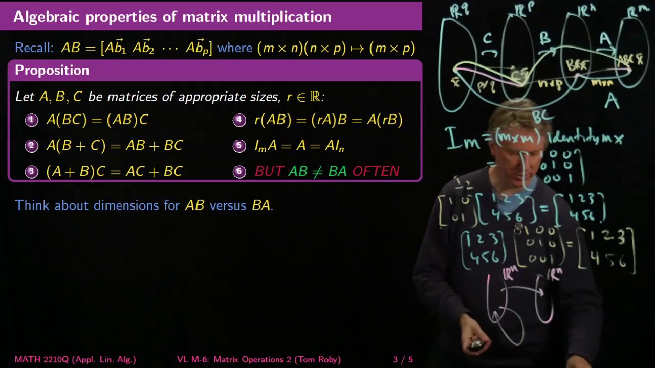
Associative and distributive properties of matrix multiplication and addition; multiplication by the identity matrix; definition of the transpose of a matrix; transpose of the transpose, transpose of a sum, transpose of a product
Matrix-scalar multiplication is commutative, associative, and distributive. math.la.t.mat.scalar.mult.commut_assoc
Matrix multiplication is distributive over matrix addition. math.la.t.mat.mult.distributive
The identity matrix is the identity for matrix multiplication. math.la.t.mat.mult.identity
Definition of transpose of a matrix math.la.d.mat.transpose
Matrix transpose is an involution. math.la.t.mat.transpose.involution
The transpose of a product of matrices is the product of the transposes in reverse order. math.la.t.mat.mult.transpose
- Created On
- August 25th, 2017
- 7 years ago
- Views
- 2
- Type
- Video
- Language
- English
- Content Type
- text/html; charset=utf-8
In this section we specialize further and consider matrices with equal numbers of rows and columns, which when considered as coefficient matrices lead to systems with equal numbers of equations and variables. We will see in the second half of the course (Chapter D, Chapter E, Chapter LT, Chapter R) that these matrices are especially important.
Definition of identity matrix math.la.d.mat.identity
- License
- GFDL-1.2
- Submitted At
- September 11th, 2017
- 7 years ago
- Views
- 2
- Type
- Textbook
- Language
- English
- Content Type
- text/html
In this section we will back up and start simple. We begin with a definition of a totally general set of matrices, and see where that takes us.
Definition of transpose of a matrix math.la.d.mat.transpose
- License
- GFDL-1.2
- Submitted At
- September 11th, 2017
- 7 years ago
- Views
- 2
- Type
- Textbook
- Language
- English
- Content Type
- text/html
In this section we will back up and start simple. We begin with a definition of a totally general set of matrices, and see where that takes us.
Definition of matrix-scalar multiplication math.la.d.mat.scalar.mult
- License
- GFDL-1.2
- Submitted At
- September 11th, 2017
- 7 years ago
- Views
- 2
- Type
- Textbook
- Language
- English
- Content Type
- text/html
In this section we will back up and start simple. We begin with a definition of a totally general set of matrices, and see where that takes us.
Matrix transpose is an involution. math.la.t.mat.transpose.involution
- License
- GFDL-1.2
- Submitted At
- September 11th, 2017
- 7 years ago
- Views
- 3
- Type
- Textbook
- Language
- English
- Content Type
- text/html
In this section we will back up and start simple. We begin with a definition of a totally general set of matrices, and see where that takes us.
Definition of sum of matrices math.la.d.mat.sum
- License
- GFDL-1.2
- Submitted At
- September 11th, 2017
- 7 years ago
- Views
- 2
- Type
- Textbook
- Language
- English
- Content Type
- text/html
In this section we will back up and start simple. We begin with a definition of a totally general set of matrices, and see where that takes us.
Definition of the diagonal of a matrix math.la.d.mat.thediagonal
- License
- GFDL-1.2
- Submitted At
- September 11th, 2017
- 7 years ago
- Views
- 3
- Type
- Textbook
- Language
- English
- Content Type
- text/html
In this section we will back up and start simple. We begin with a definition of a totally general set of matrices, and see where that takes us.
Definition of equality of matrices math.la.d.mat.equal
- License
- GFDL-1.2
- Submitted At
- September 11th, 2017
- 7 years ago
- Views
- 3
- Type
- Textbook
- Language
- English
- Content Type
- text/html
We know how to add vectors and how to multiply them by scalars. Together, these operations give us the possibility of making linear combinations. Similarly, we know how to add matrices and how to multiply matrices by scalars. In this section we mix all these ideas together and produce an operation known as matrix multiplication. This will lead to some results that are both surprising and central. We begin with a definition of how to multiply a vector by a matrix.
Definition of matrix multiplication in terms of column vectors math.la.d.mat.mult.col
- License
- GFDL-1.2
- Submitted At
- September 11th, 2017
- 7 years ago
- Views
- 3
- Type
- Textbook
- Language
- English
- Content Type
- text/html
We know how to add vectors and how to multiply them by scalars. Together, these operations give us the possibility of making linear combinations. Similarly, we know how to add matrices and how to multiply matrices by scalars. In this section we mix all these ideas together and produce an operation known as matrix multiplication. This will lead to some results that are both surprising and central. We begin with a definition of how to multiply a vector by a matrix.
Matrix multiplication is associative. math.la.t.mat.mult.assoc
- License
- GFDL-1.2
- Submitted At
- September 11th, 2017
- 7 years ago
- Views
- 3
- Type
- Textbook
- Language
- English
- Content Type
- text/html
We know how to add vectors and how to multiply them by scalars. Together, these operations give us the possibility of making linear combinations. Similarly, we know how to add matrices and how to multiply matrices by scalars. In this section we mix all these ideas together and produce an operation known as matrix multiplication. This will lead to some results that are both surprising and central. We begin with a definition of how to multiply a vector by a matrix.
The transpose of a product of matrices is the product of the transposes in reverse order. math.la.t.mat.mult.transpose
- License
- GFDL-1.2
- Submitted At
- September 11th, 2017
- 7 years ago
- Views
- 3
- Type
- Textbook
- Language
- English
- Content Type
- text/html
We know how to add vectors and how to multiply them by scalars. Together, these operations give us the possibility of making linear combinations. Similarly, we know how to add matrices and how to multiply matrices by scalars. In this section we mix all these ideas together and produce an operation known as matrix multiplication. This will lead to some results that are both surprising and central. We begin with a definition of how to multiply a vector by a matrix.
Matrix multiplication is distributive over matrix addition. math.la.t.mat.mult.distributive
- License
- GFDL-1.2
- Submitted At
- September 11th, 2017
- 7 years ago
- Views
- 3
- Type
- Textbook
- Language
- English
- Content Type
- text/html
We know how to add vectors and how to multiply them by scalars. Together, these operations give us the possibility of making linear combinations. Similarly, we know how to add matrices and how to multiply matrices by scalars. In this section we mix all these ideas together and produce an operation known as matrix multiplication. This will lead to some results that are both surprising and central. We begin with a definition of how to multiply a vector by a matrix.
The identity matrix is the identity for matrix multiplication. math.la.t.mat.mult.identity
- License
- GFDL-1.2
- Submitted At
- September 11th, 2017
- 7 years ago
- Views
- 2
- Type
- Textbook
- Language
- English
- Content Type
- text/html
This section's topic will perhaps seem out of place at first, but we will make the connection soon with eigenvalues and eigenvectors. This is also our first look at one of the central ideas of Chapter R.
Definition of diagonal matrix math.la.d.mat.diagonal
- License
- GFDL-1.2
- Submitted At
- September 11th, 2017
- 7 years ago
- Views
- 3
- Type
- Textbook
- Language
- English
- Content Type
- text/html
Definition of matrix multiplication, each entry separately math.la.d.mat.mult.coord
Example of multiplying 3x3 matrices math.la.e.mat.mult.3x3
Example of multiplying matrices math.la.e.mat.mult
XXXX
For matrices, AB=0 does not imply A=0 or B=0 in general. math.la.c.mat.mult.zero_divisor
2.2 The Inverse of a Matrix
Motivation and definition of the inverse of a matrix
Definition of matrix inverse math.la.d.mat.inv
Definition of identity matrix math.la.d.mat.identity
Matrix inverses are unique: if A and B are square matrices, then AB=I implies that A=B^-1 and B=A^-1. math.la.t.mat.inv.unique
- License
- (CC-BY-NC-SA-4.0 OR CC-BY-SA-4.0)
- Created On
- January 5th, 2017
- 8 years ago
- Views
- 3
- Type
- Video
- Timeframe
- Pre-class
- Perspective
- Introduction
- Language
- English
- Content Type
- text/html; charset=utf-8
The definition of matrix inverse is motivated by considering multiplicative inverse. The identity matrix and matrix inverse are defined.
Definition of matrix inverse math.la.d.mat.inv
Definition of identity matrix math.la.d.mat.identity
The identity matrix is the identity for matrix multiplication. math.la.t.mat.mult.identity
- Created On
- February 17th, 2017
- 7 years ago
- Views
- 2
- Type
- Video
- Timeframe
- Pre-class
- Perspective
- Introduction
- Language
- English
- Content Type
- text/html; charset=utf-8
The formula for the inverse of a 2x2 matrix is derived. (need tag for that formula)

Formula for the determinant of a 2-by-2 matrix. math.la.t.mat.det.2x2
- Created On
- February 17th, 2017
- 7 years ago
- Views
- 2
- Type
- Video
- Timeframe
- Pre-class
- Perspective
- Introduction
- Language
- English
- Content Type
- text/html; charset=utf-8
Matrix inverses are motivated as a way to solve a linear system. The general algorithm of finding an inverse by row reducing an augmented matrix is described, and then implemented for a 3x3 matrix. Useful facts about inverses are stated and then illustrated with sample 2x2 matrices. (put first: need Example of finding the inverse of a 3-by-3 matrix by row reducing the augmented matrix)

The inverse of a matrix (if it exists) can be found by row reducing the matrix augmented by the identity matrix. math.la.t.mat.inv.augmented
The inverse of a matrix can be used to solve a linear system. math.la.t.eqn.mat.inv
- Created On
- February 19th, 2017
- 7 years ago
- Views
- 3
- Type
- Video
- Timeframe
- Pre-class
- Perspective
- Introduction
- Language
- English
- Content Type
- text/html; charset=utf-8
Suggested classroom activities on matrix inverses.

Definition of matrix inverse math.la.d.mat.inv
The inverse of a matrix (if it exists) can be found by row reducing the matrix augmented by the identity matrix. math.la.t.mat.inv.augmented
- Created On
- February 19th, 2017
- 7 years ago
- Views
- 2
- Type
- Handout
- Timeframe
- In-class
- Perspective
- Introduction
- Language
- English
- Content Type
- text/html; charset=utf-8
This is a guided discovery of the formula for Lagrange Interpolation, which lets you find the formula for a polynomial which passes through a given set of points.

Definition of matrix inverse math.la.d.mat.inv
The inverse of a matrix can be used to solve a linear system. math.la.t.eqn.mat.inv
Definition of change of corrdinates matrix between two bases, arbitrary vector space math.la.d.vsp.change_of_basis.arb
The set of all polynomials of degree at most n is a vector space. math.la.t.vsp.change_of_basis.arb
Definition of linear transformation, arbitrary vector space math.la.d.lintrans.arb
- Created On
- June 8th, 2017
- 7 years ago
- Views
- 2
- Type
- Handout
- Perspective
- Application
- Language
- English
- Content Type
- text/html; charset=utf-8
Statements that are equivalent to a square matrix being invertible; examples.

Equivalence theorem: the matrix A row-reduces to the identity matrix. math.la.t.equiv.identity
The inverse of a matrix (if it exists) can be found by row reducing the matrix augmented by the identity matrix. math.la.t.mat.inv.augmented
Equivalence theorem: the matrix A has a left inverse. math.la.t.equiv.inv.left
Equivalence theorem: the matrix A has a right inverse. math.la.t.equiv.inv.right
Matrix inverse is an involution. math.la.t.mat.inv.involution
The inverse of a matrix can be used to solve a linear system. math.la.t.eqn.mat.inv
Definition of nonsingular matrix: matrix is invertible math.la.d.mat.nonsingular.inv
Definition of matrix inverse math.la.d.mat.inv
- Created On
- August 21st, 2017
- 7 years ago
- Views
- 3
- Type
- Video
- Language
- English
- Content Type
- text/html; charset=utf-8
Definition of the inverse of a matrix, examples, uniqueness; formula for the inverse of a 2x2 matrix; determinant of a 2x2 matrix; using the inverse to solve a system of linear equations.

Definition of matrix inverse math.la.d.mat.inv
Definition of nonsingular matrix: matrix is invertible math.la.d.mat.nonsingular.inv
Formula for the determinant of a 2-by-2 matrix. math.la.t.mat.det.2x2
The inverse of a matrix can be used to solve a linear system. math.la.t.eqn.mat.inv
- Created On
- August 22nd, 2017
- 7 years ago
- Views
- 4
- Type
- Video
- Language
- English
- Content Type
- text/html; charset=utf-8
Properties of matrix inversion: inverse of the inverse, inverse of the transpose, inverse of a product; elementary matrices and corresponding row operations; a matrix is invertible if and only if it is row-equivalent to the identity matrix; row-reduction algorithm for computing matrix inverse

The inverse of a matrix (if it exists) can be found by row reducing the matrix augmented by the identity matrix. math.la.t.mat.inv.augmented
Matrix inverse is an involution. math.la.t.mat.inv.involution
For n-by-n invertible matrices A and B, the product AB is invertible, and (AB)^-1=B^-1 A^-1. math.la.t.mat.inv.shoesandsocks
Matrix transpose commutes with matrix inverse. math.la.t.mat.inv.transpose
Definition of elementary matrix math.la.d.mat.elementary
Row operations are given by multiplication by elementary matrices. math.la.d.mat.mult.elementary
Elementary matrices are invertible. math.la.d.mat.elementary.inv
Equivalence theorem: the matrix A row-reduces to the identity matrix. math.la.t.equiv.identity
- Created On
- August 25th, 2017
- 7 years ago
- Views
- 3
- Type
- Video
- Language
- English
- Content Type
- text/html; charset=utf-8
In this section we specialize further and consider matrices with equal numbers of rows and columns, which when considered as coefficient matrices lead to systems with equal numbers of equations and variables. We will see in the second half of the course (Chapter D, Chapter E, Chapter LT, Chapter R) that these matrices are especially important.
Definition of nonsingular matrix: the associated homogeneous linear system has only the trivial solution math.la.d.mat.nonsingular.z
Definition of singular matrix math.la.d.mat.singular
- License
- GFDL-1.2
- Submitted At
- September 11th, 2017
- 7 years ago
- Views
- 3
- Type
- Textbook
- Language
- English
- Content Type
- text/html
In this section we specialize further and consider matrices with equal numbers of rows and columns, which when considered as coefficient matrices lead to systems with equal numbers of equations and variables. We will see in the second half of the course (Chapter D, Chapter E, Chapter LT, Chapter R) that these matrices are especially important.
Equivalence theorem: the matrix A row-reduces to the identity matrix. math.la.t.equiv.identity
- License
- GFDL-1.2
- Submitted At
- September 11th, 2017
- 7 years ago
- Views
- 2
- Type
- Textbook
- Language
- English
- Content Type
- text/html
The inverse of a square matrix, and solutions to linear systems with square coefficient matrices, are intimately connected.
Definition of matrix inverse math.la.d.mat.inv
math.la.d.mat.invertible
- License
- GFDL-1.2
- Submitted At
- September 11th, 2017
- 7 years ago
- Views
- 2
- Type
- Textbook
- Language
- English
- Content Type
- text/html
The inverse of a square matrix, and solutions to linear systems with square coefficient matrices, are intimately connected.
Matrix transpose commutes with matrix inverse. math.la.t.mat.inv.transpose
- License
- GFDL-1.2
- Submitted At
- September 11th, 2017
- 7 years ago
- Views
- 3
- Type
- Textbook
- Language
- English
- Content Type
- text/html
We saw in Theorem CINM that if a square matrix \(A\) is nonsingular, then there is a matrix \(B\) so that \(AB=I_n\text{.}\) In other words, \(B\) is halfway to being an inverse of \(A\text{.}\) We will see in this section that \(B\) automatically fulfills the second condition (\(BA=I_n\)). Example MWIAA showed us that the coefficient matrix from Archetype A had no inverse. Not coincidentally, this coefficient matrix is singular. We will make all these connections precise now. Not many examples or definitions in this section, just theorems.
The inverse of a matrix can be used to solve a linear system. math.la.t.eqn.mat.inv
- License
- GFDL-1.2
- Submitted At
- September 11th, 2017
- 7 years ago
- Views
- 3
- Type
- Textbook
- Language
- English
- Content Type
- text/html
The inverse of a square matrix, and solutions to linear systems with square coefficient matrices, are intimately connected.
Matrix inverse is an involution. math.la.t.mat.inv.involution
- License
- GFDL-1.2
- Submitted At
- September 11th, 2017
- 7 years ago
- Views
- 2
- Type
- Textbook
- Language
- English
- Content Type
- text/html
Before we define the determinant of a matrix, we take a slight detour to introduce elementary matrices. These will bring us back to the beginning of the course and our old friend, row operations.
Formula for the determinant of a 2-by-2 matrix. math.la.t.mat.det.2x2
- License
- GFDL-1.2
- Submitted At
- September 11th, 2017
- 7 years ago
- Views
- 3
- Type
- Textbook
- Language
- English
- Content Type
- text/html
The inverse of a square matrix, and solutions to linear systems with square coefficient matrices, are intimately connected.
For n-by-n invertible matrices A and B, the product AB is invertible, and (AB)^-1=B^-1 A^-1. math.la.t.mat.inv.shoesandsocks
- License
- GFDL-1.2
- Submitted At
- September 11th, 2017
- 7 years ago
- Views
- 3
- Type
- Textbook
- Language
- English
- Content Type
- text/html
The inverse of a square matrix, and solutions to linear systems with square coefficient matrices, are intimately connected.
The inverse of a matrix (if it exists) can be found by row reducing the matrix augmented by the identity matrix. math.la.t.mat.inv.augmented
- License
- GFDL-1.2
- Submitted At
- September 11th, 2017
- 7 years ago
- Views
- 3
- Type
- Textbook
- Language
- English
- Content Type
- text/html
Before we define the determinant of a matrix, we take a slight detour to introduce elementary matrices. These will bring us back to the beginning of the course and our old friend, row operations.
Elementary matrices are invertible. math.la.d.mat.elementary.inv
- License
- GFDL-1.2
- Submitted At
- September 11th, 2017
- 7 years ago
- Views
- 2
- Type
- Textbook
- Language
- English
- Content Type
- text/html
Before we define the determinant of a matrix, we take a slight detour to introduce elementary matrices. These will bring us back to the beginning of the course and our old friend, row operations.
Definition of elementary matrix math.la.d.mat.elementary
- License
- GFDL-1.2
- Submitted At
- September 11th, 2017
- 7 years ago
- Views
- 2
- Type
- Textbook
- Language
- English
- Content Type
- text/html
math.la.t.mat.inv.2by2
math.la.t.equiv.inverse
2.3 Characterizations of Invertible Matrices
Motivation and definition of the inverse of a matrix
Definition of matrix inverse math.la.d.mat.inv
Definition of identity matrix math.la.d.mat.identity
Matrix inverses are unique: if A and B are square matrices, then AB=I implies that A=B^-1 and B=A^-1. math.la.t.mat.inv.unique
- License
- (CC-BY-NC-SA-4.0 OR CC-BY-SA-4.0)
- Created On
- January 5th, 2017
- 8 years ago
- Views
- 3
- Type
- Video
- Timeframe
- Pre-class
- Perspective
- Introduction
- Language
- English
- Content Type
- text/html; charset=utf-8
Statements that are equivalent to a square matrix being invertible; examples.
Equivalence theorem: the matrix A row-reduces to the identity matrix. math.la.t.equiv.identity
The inverse of a matrix (if it exists) can be found by row reducing the matrix augmented by the identity matrix. math.la.t.mat.inv.augmented
Equivalence theorem: the matrix A has a left inverse. math.la.t.equiv.inv.left
Equivalence theorem: the matrix A has a right inverse. math.la.t.equiv.inv.right
Matrix inverse is an involution. math.la.t.mat.inv.involution
The inverse of a matrix can be used to solve a linear system. math.la.t.eqn.mat.inv
Definition of nonsingular matrix: matrix is invertible math.la.d.mat.nonsingular.inv
Definition of matrix inverse math.la.d.mat.inv
- Created On
- August 21st, 2017
- 7 years ago
- Views
- 3
- Type
- Video
- Language
- English
- Content Type
- text/html; charset=utf-8
We have seen that linear transformations whose domain and codomain are vector spaces of columns vectors have a close relationship with matrices (Theorem MBLT, Theorem MLTCV). In this section, we will extend the relationship between matrices and linear transformations to the setting of linear transformations between abstract vector spaces.
Equivalence theorem: the linear transformation given by T(x)=Ax has an inverse. math.la.t.equiv.lintrans.inv
- License
- GFDL-1.2
- Submitted At
- September 11th, 2017
- 7 years ago
- Views
- 2
- Type
- Textbook
- Language
- English
- Content Type
- text/html
math.la.t.equiv.lintrans.onetoone
math.la.t.equiv.lintrans.onto
Equivalence theorem: the transpose of the matrix A has an inverse. math.la.t.equiv.transpose.inv
Definition of invertible linear transformation, coordinate vector space math.la.d.lintrans.invertible.coord
A matrix is called ill-conditioned if it is nearly singular math.la.c.mat.illconditioned
The condition number of matrix measures how close it is to being singular math.la.c.mat.conditionnumber
math.la.d.mat.triangular.upper.exer
math.la.d.mat.triangular.lower.exer
2.4 Partitioned Matrices
Definition of block/partitioned matrix math.la.d.mat.block
Multiplication of block/partitioned matrices math.la.c.mat.mult.block
Matrix multiplication can be viewed as the dot product of a row vector of column vectors with a column vector of row vectors math.la.t.mat.mult.row.col
Definition of block diagonal matrix math.la.d.mat.block_diagonal
2.5 Matrix Factorizations
Definition of LU decomposition math.la.d.mat.lu
Algorithm for computing an LU decomposition math.la.t.mat.lu
math.la.d.mat.lu.reduced.exer
math.la.d.mat.rank_factorization.exer
math.la.d.mat.qr.exer
math.la.d.mat.svd.exer
math.la.d.mat.band.exer
2.6 The Leontief Input-Output Model
2.7 Applications to Computer Graphics
2.8 Subspaces of Rn
Basis theorem: for an n-dimensional vector space any linearly independent set with n elements is a basis, as is any spanning set with n elements; dimension of the column space of a matrix equals the number of pivot columns of the matrix; dimension of the null space of a matrix equals the number of free variables of the matrix

Any linearly independent set can be expanded to a basis for the (sub)space, arbitrary vector space. math.la.t.vsp.linindep.basis.arb
If a vector space has dimension n, then any subset of n vectors that is linearly independent must be a basis, arbitrary vector space. math.la.t.vsp.dim.linindep.arb
If a vector space has dimension n, then any subset set of n vectors that spans the space must be a basis, arbitrary vector space. math.la.t.vsp.dim.span.arb
The dimension of a subspace is less than or equal to the dimension of the whole space, arbitrary vector space. math.la.t.vsp.subspace.dim.arb
The pivot columns of a matrix are a basis for the column space. math.la.t.mat.col_space.pivot
- Created On
- August 25th, 2017
- 7 years ago
- Views
- 4
- Type
- Video
- Language
- English
- Content Type
- text/html; charset=utf-8
The pivot columns of a matrix form a basis for its column space; nullspace of a matrix equals the nullspace of its reduced row-echelon form.

The pivot columns of a matrix are a basis for the column space. math.la.t.mat.col_space.pivot
- Created On
- August 25th, 2017
- 7 years ago
- Views
- 4
- Type
- Video
- Language
- English
- Content Type
- text/html; charset=utf-8
Definition of the column space of a matrix; column space is a subspace; comparison to the null space; definition of a linear transformation between vector spaces; definition of kernel and range of a linear transformation

Definition of column space of a matrix math.la.d.mat.col_space
Definition of linear transformation, arbitrary vector space math.la.d.lintrans.arb
Definition of kernel of linear transformation, arbitrary vector space math.la.d.lintrans.kernel.arb
Definition of range of linear transformation, arbitrary vector space math.la.d.lintrans.range.arb
- Created On
- August 25th, 2017
- 7 years ago
- Views
- 3
- Type
- Video
- Language
- English
- Content Type
- text/html; charset=utf-8
In this section we specialize to systems of linear equations where every equation has a zero as its constant term. Along the way, we will begin to express more and more ideas in the language of matrices and begin a move away from writing out whole systems of equations. The ideas initiated in this section will carry through the remainder of the course.
Definition of matrix null space (right) math.la.d.mat.null_space.right
- License
- GFDL-1.2
- Submitted At
- September 11th, 2017
- 7 years ago
- Views
- 2
- Type
- Textbook
- Language
- English
- Content Type
- text/html
In this section we define a couple more operations with vectors, and prove a few theorems. At first blush these definitions and results will not appear central to what follows, but we will make use of them at key points in the remainder of the course (such as Section MINM, Section OD). Because we have chosen to use \(\complexes\) as our set of scalars, this subsection is a bit more, uh, … complex than it would be for the real numbers. We will explain as we go along how things get easier for the real numbers \({\mathbb R}\text{.}\) If you have not already, now would be a good time to review some of the basic properties of arithmetic with complex numbers described in Section CNO. With that done, we can extend the basics of complex number arithmetic to our study of vectors in \(\complex{m}\text{.}\)
Definition of the standard basis of R^n (or C^n) math.la.d.vsp.basis.standard.rncn
Definition of unit vector, coordinate setting math.la.d.vec.unit.coord
- License
- GFDL-1.2
- Submitted At
- September 11th, 2017
- 7 years ago
- Views
- 2
- Type
- Textbook
- Language
- English
- Content Type
- text/html
A matrix-vector product (Definition MVP) is a linear combination of the columns of the matrix and this allows us to connect matrix multiplication with systems of equations via Theorem SLSLC. Row operations are linear combinations of the rows of a matrix, and of course, reduced row-echelon form (Definition RREF) is also intimately related to solving systems of equations. In this section we will formalize these ideas with two key definitions of sets of vectors derived from a matrix.
The pivot columns of a matrix are a basis for the column space. math.la.t.mat.col_space.pivot
- License
- GFDL-1.2
- Submitted At
- September 11th, 2017
- 7 years ago
- Views
- 4
- Type
- Textbook
- Language
- English
- Content Type
- text/html
A subspace is a vector space that is contained within another vector space. So every subspace is a vector space in its own right, but it is also defined relative to some other (larger) vector space. We will discover shortly that we are already familiar with a wide variety of subspaces from previous sections.
The null space of a matrix is a subspace of R^n (or C^n). math.la.t.mat.null_space.rncn
- License
- GFDL-1.2
- Submitted At
- September 11th, 2017
- 7 years ago
- Views
- 2
- Type
- Textbook
- Language
- English
- Content Type
- text/html
A matrix-vector product (Definition MVP) is a linear combination of the columns of the matrix and this allows us to connect matrix multiplication with systems of equations via Theorem SLSLC. Row operations are linear combinations of the rows of a matrix, and of course, reduced row-echelon form (Definition RREF) is also intimately related to solving systems of equations. In this section we will formalize these ideas with two key definitions of sets of vectors derived from a matrix.
Definition of column space of a matrix math.la.d.mat.col_space
- License
- GFDL-1.2
- Submitted At
- September 11th, 2017
- 7 years ago
- Views
- 3
- Type
- Textbook
- Language
- English
- Content Type
- text/html
Definition of subspace, coordinate vector space math.la.d.vsp.subspace.coord
Definition of subspace spanned by a set of a set of vectors, coordinate vector space math.la.d.vec.span.subspace.coord
The column space of an m-by-n matrix is a subspace of R^m (or C^m) math.la.t.mat.col_space.rncn
Definition of basis of a vector space (or subspace), coordinate vector space math.la.d.vsp.basis.coord
2.9 Dimension and Rank
Students answer multiple questions on the rank and dimension of the null space in a variety of situations to discover the connection between these dimensions leading to the Rank-Nullity Theorem.
If A is a matrix, then the rank of A plus the nullity of A equals the number of columns of A. math.la.t.mat.ranknullity
- Created On
- June 9th, 2017
- 7 years ago
- Views
- 2
- Type
- Handout
- Timeframe
- In-class
- Language
- English
- Content Type
- text/html; charset=utf-8
Representation (unique) of a vector in terms of a basis for a vector space yields coordinates relative to the basis; change of basis and corresponding change of coordinate matrix

Each vector can be written uniquely as a linear combination of vectors from a given basis. math.la.t.vsp.basis.coord.unique
Definition of coordinates relative to a given basis, arbitrary vector space math.la.d.vsp.basis.relative.arb
Definition of change-of-coordinates matrix relative to a given basis of R^n (or C^n) math.la.d.vsp.basis.coord.change.rncn
Definition of coordinates relative to a given basis, coordinate vector space math.la.d.vsp.basis.relative.coord
- Created On
- August 25th, 2017
- 7 years ago
- Views
- 3
- Type
- Video
- Language
- English
- Content Type
- text/html; charset=utf-8
In this section we specialize further and consider matrices with equal numbers of rows and columns, which when considered as coefficient matrices lead to systems with equal numbers of equations and variables. We will see in the second half of the course (Chapter D, Chapter E, Chapter LT, Chapter R) that these matrices are especially important.
Equivalence theorem: the null space of the matrix A is {0}. math.la.t.equiv.nullspace
- License
- GFDL-1.2
- Submitted At
- September 11th, 2017
- 7 years ago
- Views
- 3
- Type
- Textbook
- Language
- English
- Content Type
- text/html
Almost every vector space we have encountered has been infinite in size (an exception is Example VSS). But some are bigger and richer than others. Dimension, once suitably defined, will be a measure of the size of a vector space, and a useful tool for studying its properties. You probably already have a rough notion of what a mathematical definition of dimension might be — try to forget these imprecise ideas and go with the new ones given here.
Equivalence theorem: the matrix A has rank n. math.la.t.equiv.rank
Equivalence theorem: the nullity of the matrix A is zero. math.la.t.equiv.nullity
- License
- GFDL-1.2
- Submitted At
- September 11th, 2017
- 7 years ago
- Views
- 2
- Type
- Textbook
- Language
- English
- Content Type
- text/html
Almost every vector space we have encountered has been infinite in size (an exception is Example VSS). But some are bigger and richer than others. Dimension, once suitably defined, will be a measure of the size of a vector space, and a useful tool for studying its properties. You probably already have a rough notion of what a mathematical definition of dimension might be — try to forget these imprecise ideas and go with the new ones given here.
Definition of rank of a matrix math.la.d.mat.rank
- License
- GFDL-1.2
- Submitted At
- September 11th, 2017
- 7 years ago
- Views
- 2
- Type
- Textbook
- Language
- English
- Content Type
- text/html
Almost every vector space we have encountered has been infinite in size (an exception is Example VSS). But some are bigger and richer than others. Dimension, once suitably defined, will be a measure of the size of a vector space, and a useful tool for studying its properties. You probably already have a rough notion of what a mathematical definition of dimension might be — try to forget these imprecise ideas and go with the new ones given here.
If A is a matrix, then the rank of A plus the nullity of A equals the number of columns of A. math.la.t.mat.ranknullity
- License
- GFDL-1.2
- Submitted At
- September 11th, 2017
- 7 years ago
- Views
- 3
- Type
- Textbook
- Language
- English
- Content Type
- text/html
Definition of dimension of a vector space (or subspace), coordinate vector space math.la.d.vsp.dim.coord
If a vector space has dimension n, then any subset set of n vectors that spans the space must be a basis, coordinate vector space. math.la.t.vsp.dim.span.coord
If a vector space has dimension n, then any subset of n vectors that is linearly independent must be a basis, coordinate vector space. math.la.t.vsp.dim.linindep.coord
Equivalence theorem: the dimension of the column space of A is n. math.la.t.equiv.col.dim
Supplementary Exercises
3 Determinants
3.1 Introduction to Determinants
The effect of row operations on the determinant of a matrix; computing determinants via row reduction; a square matrix is invertible if and only if its determinant is nonzero.

Theorem describing the effect of elementary row operations on the determinant of a matrix. math.la.t.mat.det.elementaryoperations
Equivalence theorem: the determinant of A is nonzero. math.la.t.equiv.det
The determinant of a triangular matrix is the product of the entries on the diagonal. math.la.t.mat.det.trianglar
- Created On
- August 22nd, 2017
- 7 years ago
- Views
- 4
- Type
- Video
- Language
- English
- Content Type
- text/html; charset=utf-8
Before we define the determinant of a matrix, we take a slight detour to introduce elementary matrices. These will bring us back to the beginning of the course and our old friend, row operations.
Definition of determinant of a matrix as a cofactor expansion across the first row math.la.d.mat.det.cofactor
- License
- GFDL-1.2
- Submitted At
- September 11th, 2017
- 7 years ago
- Views
- 3
- Type
- Textbook
- Language
- English
- Content Type
- text/html
Formula for the determinant of a 3-by-3 matrix. math.la.t.mat.det.3x3
The determinant of a matrix can be computed as a cofactor expansion across any row or down any column. math.la.t.mat.det.cofactor
3.2 Properties of Determinants
The effect of row operations on the determinant of a matrix; computing determinants via row reduction; a square matrix is invertible if and only if its determinant is nonzero.
Theorem describing the effect of elementary row operations on the determinant of a matrix. math.la.t.mat.det.elementaryoperations
Equivalence theorem: the determinant of A is nonzero. math.la.t.equiv.det
The determinant of a triangular matrix is the product of the entries on the diagonal. math.la.t.mat.det.trianglar
- Created On
- August 22nd, 2017
- 7 years ago
- Views
- 4
- Type
- Video
- Language
- English
- Content Type
- text/html; charset=utf-8
Determinant of the transpose equals the determinant of the original matrix; rescaling a column rescales the determinant by the same factor; interchanging two columns changes the sign of the determinant; adding multiple of one column to another leaves determinant unchanged; determinant of the product of two matrices equals product of the two determinants

A matrix and its transpose have the same determinant. math.la.t.mat.det.transpose
If A and B are n-by-n matrices, then det(AB)=det(A)det(B). math.la.t.mat.det.product
Theorem describing the effect of elementary row operations on the determinant of a matrix. math.la.t.mat.det.elementaryoperations
- Created On
- August 25th, 2017
- 7 years ago
- Views
- 3
- Type
- Video
- Language
- English
- Content Type
- text/html; charset=utf-8
We have seen how to compute the determinant of a matrix, and the incredible fact that we can perform expansion about any row or column to make this computation. In this largely theoretical section, we will state and prove several more intriguing properties about determinants. Our main goal will be the two results in Theorem SMZD and Theorem DRMM, but more specifically, we will see how the value of a determinant will allow us to gain insight into the various properties of a square matrix.
Equivalence theorem: the determinant of A is nonzero. math.la.t.equiv.det
- License
- GFDL-1.2
- Submitted At
- September 11th, 2017
- 7 years ago
- Views
- 2
- Type
- Textbook
- Language
- English
- Content Type
- text/html
We have seen how to compute the determinant of a matrix, and the incredible fact that we can perform expansion about any row or column to make this computation. In this largely theoretical section, we will state and prove several more intriguing properties about determinants. Our main goal will be the two results in Theorem SMZD and Theorem DRMM, but more specifically, we will see how the value of a determinant will allow us to gain insight into the various properties of a square matrix.
Theorem describing the determinants of elementary matrices. math.la.t.mat.elementary.det
- License
- GFDL-1.2
- Submitted At
- September 11th, 2017
- 7 years ago
- Views
- 3
- Type
- Textbook
- Language
- English
- Content Type
- text/html
We have seen how to compute the determinant of a matrix, and the incredible fact that we can perform expansion about any row or column to make this computation. In this largely theoretical section, we will state and prove several more intriguing properties about determinants. Our main goal will be the two results in Theorem SMZD and Theorem DRMM, but more specifically, we will see how the value of a determinant will allow us to gain insight into the various properties of a square matrix.
If A and B are n-by-n matrices, then det(AB)=det(A)det(B). math.la.t.mat.det.product
- License
- GFDL-1.2
- Submitted At
- September 11th, 2017
- 7 years ago
- Views
- 3
- Type
- Textbook
- Language
- English
- Content Type
- text/html
Before we define the determinant of a matrix, we take a slight detour to introduce elementary matrices. These will bring us back to the beginning of the course and our old friend, row operations.
A matrix and its transpose have the same determinant. math.la.t.mat.det.transpose
- License
- GFDL-1.2
- Submitted At
- September 11th, 2017
- 7 years ago
- Views
- 3
- Type
- Textbook
- Language
- English
- Content Type
- text/html
The determinant of a matrix can be expressed as a product of the diagonal entries in a non-scaled echelon form. math.la.t.mat.det.echelon
3.3 Cramer's Rule, Volume, and Linear Transformations
Cramer's rule math.la.t.cramer
Definition of adjugate/classical adjoint of a matrix math.la.d.mat.classicaladjoint
math.la.t.mat.inv.cofactor
The determinant of a matrix measures the area/volume of the parallelogram/parallelipiped determined by its columns. math.la.t.mat.det.col.volume
The determinant of the matrix of a linear transformation is the factor by which the area/volume changes. math.la.t.lintrans.det.volume
math.la.d.mat.vandermonde.exer
Supplementary Exercises
4 Vector Spaces
4.1 Vector Spaces and Subspaces
This video kicks off the series of videos on vector spaces. We begin by summarizing the essential properties of R^n.

Axioms of a vector space, arbitrary vector space math.la.d.vsp.axioms.arb
- License
- CC-BY-SA-4.0
- Created On
- January 1st, 2017
- 8 years ago
- Views
- 3
- Type
- Video
- Perspective
- Introduction
- Language
- English
- Content Type
- text/html; charset=utf-8
In this video we continue to list the properties of R^n. The 10 properties listed in this video and the previous video will be used to define a general vecto...

Axioms of a vector space, arbitrary vector space math.la.d.vsp.axioms.arb
- License
- CC-BY-SA-4.0
- Created On
- December 28th, 2016
- 8 years ago
- Views
- 3
- Type
- Video
- Perspective
- Introduction
- Language
- English
- Content Type
- text/html; charset=utf-8
The concept of a vector space is somewhat abstract, and under this definition, a lot of objects such as polynomials, functions, etc., can be considered as vectors. This video explains the definition of a general vector space. In later videos we will look at more examples.

Axioms of a vector space, arbitrary vector space math.la.d.vsp.axioms.arb
- License
- CC-BY-SA-4.0
- Created On
- January 1st, 2017
- 8 years ago
- Views
- 2
- Type
- Video
- Perspective
- Introduction
- Language
- English
- Content Type
- text/html; charset=utf-8
Preliminaries: 1. What is a subset? 2. How to verify a set is a subset of another set? 3. Notations and language of set theory related to subsets. In this video, we introduce the definition of a subspace. We go through a preliminary example to figure out what do subspaces of R^2 look like, and we will continue to talk about how to verify a subset of a vector space is a subspace in later videos.
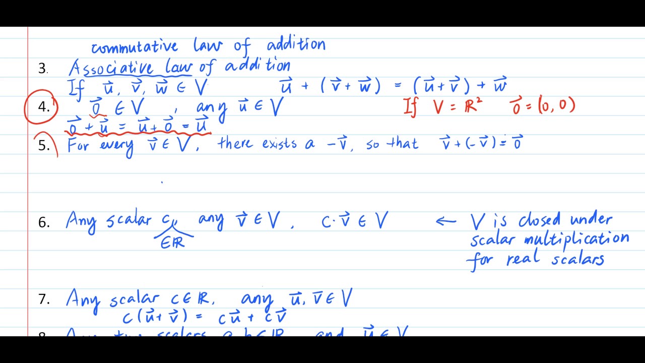
Definition of subspace, arbitrary vector space math.la.d.vsp.subspace.arb
- License
- CC-BY-SA-4.0
- Created On
- January 3rd, 2017
- 8 years ago
- Views
- 3
- Type
- Video
- Perspective
- Introduction
- Language
- English
- Content Type
- text/html; charset=utf-8
In this video, I'll explain why we only need to test 2 axioms (among the 10 axioms in the definition of a vector space) when figuring out if a subset is a subspace.
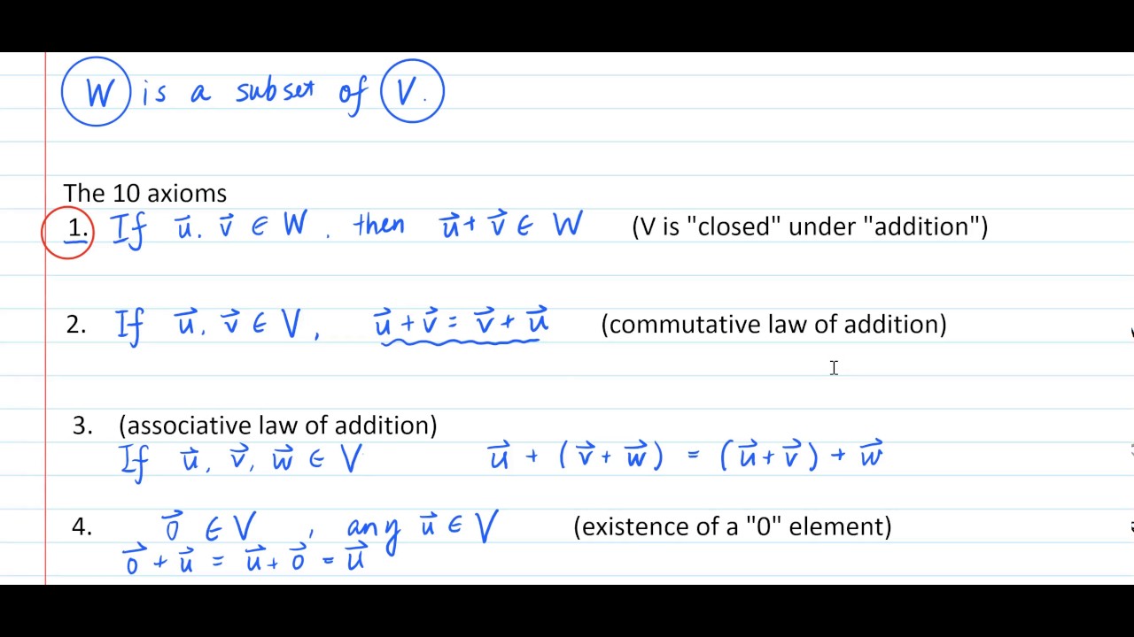
Definition of subspace, arbitrary vector space math.la.d.vsp.subspace.arb
- License
- CC-BY-SA-4.0
- Created On
- June 9th, 2017
- 7 years ago
- Views
- 3
- Type
- Video
- Timeframe
- Pre-class
- Perspective
- Introduction
- Language
- English
- Content Type
- text/html; charset=utf-8
Definition of a (real) vector space; properties of the zero vector and the additive inverse in relation to scalar multiplication

Axioms of a vector space, arbitrary vector space math.la.d.vsp.axioms.arb
Definition of vector, arbitrary vector space math.la.d.vec.arb
Definition of vector addition, arbitrary vector space math.la.d.vec.add.arb
Definition of vector-scalar multiplication, arbitrary vector space math.la.d.vec.scalar.mult.arb
The additive inverse of a vector is called the negative of the vector. math.la.d.vsp.vector.negative
The zero scalar multiplied by any vector equals the zero vector. math.la.t.vsp.scalar.mult.z
The zero vector multiplied by any scalar equals the zero vector. math.la.t.vsp.vector.mult.z
The negative of a vector equals the vector multiplied by -1. math.la.t.vsp.vector.negative
- Created On
- August 25th, 2017
- 7 years ago
- Views
- 2
- Type
- Video
- Language
- English
- Content Type
- text/html; charset=utf-8
Definition of a vector; vector addition; scalar multiplication; visualization in R^2 and R^3; vector space axioms; linear combinations; span.
Definition of linear combination of vectors, arbitrary vector space math.la.d.vec.lincomb.arb
Example of linear combination of vectors in R^2 math.la.e.vec.lincomb.r2
Example of writing a given vector in R^3 as a linear combination of given vectors math.la.e.vec.lincomb.weight.solve.r3
- Created On
- September 3rd, 2017
- 7 years ago
- Views
- 2
- Type
- Video
- Language
- English
- Content Type
- text/html; charset=utf-8
Definition of a subspace of a vector space; examples; span of vectors is a subspace.

Definition of subspace, arbitrary vector space math.la.d.vsp.subspace.arb
Definition of subspace spaned by a set of vectors, arbitrary vector space math.la.d.vec.span.subspace.arb
Definition of zero subspace, arbitrary vector space math.la.d.vsp.subspace.z
- Created On
- September 3rd, 2017
- 7 years ago
- Views
- 2
- Type
- Video
- Language
- English
- Content Type
- text/html; charset=utf-8
In this section we present a formal definition of a vector space, which will lead to an extra increment of abstraction. Once defined, we study its most basic properties.
The negative of a vector equals the vector multiplied by -1. math.la.t.vsp.vector.negative
- License
- GFDL-1.2
- Submitted At
- September 11th, 2017
- 7 years ago
- Views
- 2
- Type
- Textbook
- Language
- English
- Content Type
- text/html
In this section we present a formal definition of a vector space, which will lead to an extra increment of abstraction. Once defined, we study its most basic properties.
math.la.e.vsp.polynomial.leq_n
- License
- GFDL-1.2
- Submitted At
- September 11th, 2017
- 7 years ago
- Views
- 3
- Type
- Textbook
- Language
- English
- Content Type
- text/html
In this section we present a formal definition of a vector space, which will lead to an extra increment of abstraction. Once defined, we study its most basic properties.
The zero scalar multiplied by any vector equals the zero vector. math.la.t.vsp.scalar.mult.z
- License
- GFDL-1.2
- Submitted At
- September 11th, 2017
- 7 years ago
- Views
- 2
- Type
- Textbook
- Language
- English
- Content Type
- text/html
A subspace is a vector space that is contained within another vector space. So every subspace is a vector space in its own right, but it is also defined relative to some other (larger) vector space. We will discover shortly that we are already familiar with a wide variety of subspaces from previous sections.
Definition of subspace, arbitrary vector space math.la.d.vsp.subspace.arb
- License
- GFDL-1.2
- Submitted At
- September 11th, 2017
- 7 years ago
- Views
- 2
- Type
- Textbook
- Language
- English
- Content Type
- text/html
In this section we present a formal definition of a vector space, which will lead to an extra increment of abstraction. Once defined, we study its most basic properties.
Definition of vector addition, arbitrary vector space math.la.d.vec.add.arb
Definition of vector-scalar multiplication, arbitrary vector space math.la.d.vec.scalar.mult.arb
Axioms of a vector space, arbitrary vector space math.la.d.vsp.axioms.arb
Definition of vector, arbitrary vector space math.la.d.vec.arb
- License
- GFDL-1.2
- Submitted At
- September 11th, 2017
- 7 years ago
- Views
- 2
- Type
- Textbook
- Language
- English
- Content Type
- text/html
In this section we present a formal definition of a vector space, which will lead to an extra increment of abstraction. Once defined, we study its most basic properties.
math.la.e.vsp.function
- License
- GFDL-1.2
- Submitted At
- September 11th, 2017
- 7 years ago
- Views
- 2
- Type
- Textbook
- Language
- English
- Content Type
- text/html
A vector space is defined as a set with two operations, meeting ten properties (Definition VS). Just as the definition of span of a set of vectors only required knowing how to add vectors and how to multiply vectors by scalars, so it is with linear independence. A definition of a linearly independent set of vectors in an arbitrary vector space only requires knowing how to form linear combinations and equating these with the zero vector. Since every vector space must have a zero vector (Property Z), we always have a zero vector at our disposal.
Definition of spanning set for a subspace, arbitrary vector space math.la.d.vsp.span.set.arb
- License
- GFDL-1.2
- Submitted At
- September 11th, 2017
- 7 years ago
- Views
- 3
- Type
- Textbook
- Language
- English
- Content Type
- text/html
In this section we present a formal definition of a vector space, which will lead to an extra increment of abstraction. Once defined, we study its most basic properties.
The zero vector multiplied by any scalar equals the zero vector. math.la.t.vsp.vector.mult.z
- License
- GFDL-1.2
- Submitted At
- September 11th, 2017
- 7 years ago
- Views
- 3
- Type
- Textbook
- Language
- English
- Content Type
- text/html
A subspace is a vector space that is contained within another vector space. So every subspace is a vector space in its own right, but it is also defined relative to some other (larger) vector space. We will discover shortly that we are already familiar with a wide variety of subspaces from previous sections.
Definition of span of a set of vectors, arbitrary vector space math.la.d.vec.span.arb
- License
- GFDL-1.2
- Submitted At
- September 11th, 2017
- 7 years ago
- Views
- 2
- Type
- Textbook
- Language
- English
- Content Type
- text/html
A subspace is a vector space that is contained within another vector space. So every subspace is a vector space in its own right, but it is also defined relative to some other (larger) vector space. We will discover shortly that we are already familiar with a wide variety of subspaces from previous sections.
Definition of linear combination of vectors, arbitrary vector space math.la.d.vec.lincomb.arb
- License
- GFDL-1.2
- Submitted At
- September 11th, 2017
- 7 years ago
- Views
- 3
- Type
- Textbook
- Language
- English
- Content Type
- text/html
math.la.math.functions.d.polynomial.degree
math.la.math.functions.d.polynomial.z
math.la.e.vsp.polynomial
math.la.t.vsp.span.arb
math.la.d.vsp.subspace.intersection.arb.exer
math.la.t.vsp.subspace.intersection.arb.exer
math.la.d.vsp.subspace.sum.arb.exer
math.la.t.vsp.subspace.sum.arb.exer
4.2 Null Spaces, Column Spaces, and Linear Transformations
Two proofs, with discussion, of the fact that an abstract linear transformation maps 0 to 0.
A linear transformation maps zero to zero. math.la.t.lintrans.z
Definition of linear transformation, arbitrary vector space math.la.d.lintrans.arb
- Created On
- February 15th, 2017
- 7 years ago
- Views
- 2
- Type
- Handout
- Timeframe
- Pre-class
- Perspective
- Proof
- Language
- English
- Content Type
- text/html; charset=utf-8
Matrices can be thought of as transforming space, and understanding how this work is crucial for understanding many other ideas that follow in linear algebra...
Definition of linear transformation, arbitrary vector space math.la.d.lintrans.arb
- License
- Unlicense
- Created On
- May 25th, 2017
- 7 years ago
- Views
- 2
- Type
- Video
- Timeframe
- Pre-class
- Perspective
- Introduction
- Language
- English
- Content Type
- text/html; charset=utf-8
This is a guided discovery of the formula for Lagrange Interpolation, which lets you find the formula for a polynomial which passes through a given set of points.
Definition of matrix inverse math.la.d.mat.inv
The inverse of a matrix can be used to solve a linear system. math.la.t.eqn.mat.inv
Definition of change of corrdinates matrix between two bases, arbitrary vector space math.la.d.vsp.change_of_basis.arb
The set of all polynomials of degree at most n is a vector space. math.la.t.vsp.change_of_basis.arb
Definition of linear transformation, arbitrary vector space math.la.d.lintrans.arb
- Created On
- June 8th, 2017
- 7 years ago
- Views
- 2
- Type
- Handout
- Perspective
- Application
- Language
- English
- Content Type
- text/html; charset=utf-8
Definition of the column space of a matrix; column space is a subspace; comparison to the null space; definition of a linear transformation between vector spaces; definition of kernel and range of a linear transformation
Definition of column space of a matrix math.la.d.mat.col_space
Definition of linear transformation, arbitrary vector space math.la.d.lintrans.arb
Definition of kernel of linear transformation, arbitrary vector space math.la.d.lintrans.kernel.arb
Definition of range of linear transformation, arbitrary vector space math.la.d.lintrans.range.arb
- Created On
- August 25th, 2017
- 7 years ago
- Views
- 3
- Type
- Video
- Language
- English
- Content Type
- text/html; charset=utf-8
Early in Chapter VS we prefaced the definition of a vector space with the comment that it was “one of the two most important definitions in the entire course.” Here comes the other. Any capsule summary of linear algebra would have to describe the subject as the interplay of linear transformations and vector spaces. Here we go.
Definition of linear transformation, arbitrary vector space math.la.d.lintrans.arb
- License
- GFDL-1.2
- Submitted At
- September 11th, 2017
- 7 years ago
- Views
- 3
- Type
- Textbook
- Language
- English
- Content Type
- text/html
math.la.d.mat.null_space.right.rep
math.la.t.mat.null_space.rncn.rep
math.la.d.mat.col_space.rep
math.la.t.mat.col_space.rncn.rep
4.3 Linearly Independent Sets; Bases
In any linearly dependent set there is always one vector that can be written as a linear combination of the others. This is the substance of the upcoming Theorem DLDS. Perhaps this will explain the use of the word “dependent.” In a linearly dependent set, at least one vector “depends” on the others (via a linear combination).
math.la.t.vsp.span.basis.rref
A set of nonzero vectors contains (as a subset) a basis for its span. math.la.t.vsp.span.basis
- License
- GFDL-1.2
- Submitted At
- September 11th, 2017
- 7 years ago
- Views
- 2
- Type
- Textbook
- Language
- English
- Content Type
- text/html
A vector space is defined as a set with two operations, meeting ten properties (Definition VS). Just as the definition of span of a set of vectors only required knowing how to add vectors and how to multiply vectors by scalars, so it is with linear independence. A definition of a linearly independent set of vectors in an arbitrary vector space only requires knowing how to form linear combinations and equating these with the zero vector. Since every vector space must have a zero vector (Property Z), we always have a zero vector at our disposal.
Definition of linearly indepentent set of vectors: if a linear combination is zero, then every coefficient is zero, arbitrary vector space. math.la.d.vec.linindep.arb
- License
- GFDL-1.2
- Submitted At
- September 11th, 2017
- 7 years ago
- Views
- 2
- Type
- Textbook
- Language
- English
- Content Type
- text/html
A vector space is defined as a set with two operations, meeting ten properties (Definition VS). Just as the definition of span of a set of vectors only required knowing how to add vectors and how to multiply vectors by scalars, so it is with linear independence. A definition of a linearly independent set of vectors in an arbitrary vector space only requires knowing how to form linear combinations and equating these with the zero vector. Since every vector space must have a zero vector (Property Z), we always have a zero vector at our disposal.
math.la.d.vec.lindep.relation.rep
math.la.d.vec.lindep.relation.trvial.rep
- License
- GFDL-1.2
- Submitted At
- September 11th, 2017
- 7 years ago
- Views
- 3
- Type
- Textbook
- Language
- English
- Content Type
- text/html
A basis of a vector space is one of the most useful concepts in linear algebra. It often provides a concise, finite description of an infinite vector space.
Definition of the standard basis of the polynomials of degree at most n math.la.d.vsp.basis.standard.leq_n
- License
- GFDL-1.2
- Submitted At
- September 11th, 2017
- 7 years ago
- Views
- 3
- Type
- Textbook
- Language
- English
- Content Type
- text/html
A basis of a vector space is one of the most useful concepts in linear algebra. It often provides a concise, finite description of an infinite vector space.
Definition of basis of a vector space (or subspace), arbitrary vector space math.la.d.vsp.basis.arb
- License
- GFDL-1.2
- Submitted At
- September 11th, 2017
- 7 years ago
- Views
- 3
- Type
- Textbook
- Language
- English
- Content Type
- text/html
Theorem: a set of vectors is linearly dependent if and only if one of the vectors can be written as a linear combination of the other vectors, arbitrary vector space. math.la.t.vec.lindep.arb
math.la.d.vsp.basis.standard.rncn.rep
Removing a linearly dependent vector from a set does not change the span of the set. math.la.t.vsp.span.lindep
math.la.t.mat.col_space.pivot.rep
4.4 Coordinate Systems
Representation (unique) of a vector in terms of a basis for a vector space yields coordinates relative to the basis; change of basis and corresponding change of coordinate matrix
Each vector can be written uniquely as a linear combination of vectors from a given basis. math.la.t.vsp.basis.coord.unique
Definition of coordinates relative to a given basis, arbitrary vector space math.la.d.vsp.basis.relative.arb
Definition of change-of-coordinates matrix relative to a given basis of R^n (or C^n) math.la.d.vsp.basis.coord.change.rncn
Definition of coordinates relative to a given basis, coordinate vector space math.la.d.vsp.basis.relative.coord
- Created On
- August 25th, 2017
- 7 years ago
- Views
- 3
- Type
- Video
- Language
- English
- Content Type
- text/html; charset=utf-8
Given a basis for a n-dimensional vector space V, the coordinate map is a linear bijection between V and R^n; definition isomorphisms between vector spaces and isomorphic vector spaces.
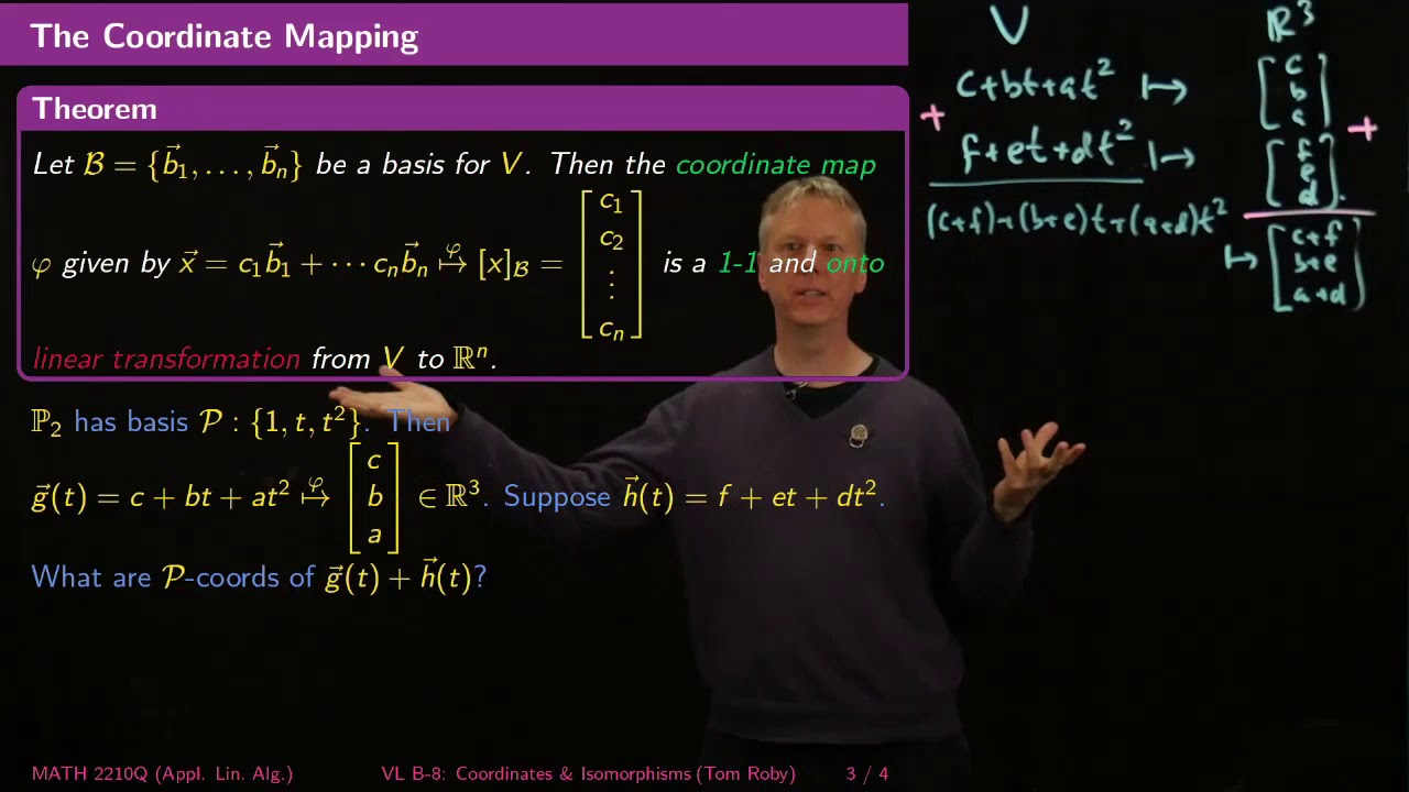
Definition of isomorphism between vector spaces math.la.d.vsp.isomorphism
The coordinate vector/mapping relative to a given basis is a bijective linear mapping to R^n (or C^n). math.la.t.vsp.basis.coord.vector.arb
- Created On
- August 25th, 2017
- 7 years ago
- Views
- 2
- Type
- Video
- Language
- English
- Content Type
- text/html; charset=utf-8
You may have noticed that many questions about elements of abstract vector spaces eventually become questions about column vectors or systems of equations. Example SM32 would be an example of this. We will make this vague idea more precise in this section.
Definition of coordinate vector/mapping relative to a given basis, arbitrary vector space math.la.d.vsp.basis.coord.vector.arb
- License
- GFDL-1.2
- Submitted At
- September 11th, 2017
- 7 years ago
- Views
- 2
- Type
- Textbook
- Language
- English
- Content Type
- text/html
In this section we will conclude our introduction to linear transformations by bringing together the twin properties of injectivity and surjectivity and consider linear transformations with both of these properties.
Definition of isomorphism between vector spaces math.la.d.vsp.isomorphism
- License
- GFDL-1.2
- Submitted At
- September 11th, 2017
- 7 years ago
- Views
- 3
- Type
- Textbook
- Language
- English
- Content Type
- text/html
A vector space is defined as a set with two operations, meeting ten properties (Definition VS). Just as the definition of span of a set of vectors only required knowing how to add vectors and how to multiply vectors by scalars, so it is with linear independence. A definition of a linearly independent set of vectors in an arbitrary vector space only requires knowing how to form linear combinations and equating these with the zero vector. Since every vector space must have a zero vector (Property Z), we always have a zero vector at our disposal.
Each vector can be written uniquely as a linear combination of vectors from a given basis. math.la.t.vsp.basis.coord.unique
- License
- GFDL-1.2
- Submitted At
- September 11th, 2017
- 7 years ago
- Views
- 3
- Type
- Textbook
- Language
- English
- Content Type
- text/html
math.la.t.vsp.basis.coord.mapping.arb
4.5 The Dimension of a Vector Space
Basis theorem: for an n-dimensional vector space any linearly independent set with n elements is a basis, as is any spanning set with n elements; dimension of the column space of a matrix equals the number of pivot columns of the matrix; dimension of the null space of a matrix equals the number of free variables of the matrix
Any linearly independent set can be expanded to a basis for the (sub)space, arbitrary vector space. math.la.t.vsp.linindep.basis.arb
If a vector space has dimension n, then any subset of n vectors that is linearly independent must be a basis, arbitrary vector space. math.la.t.vsp.dim.linindep.arb
If a vector space has dimension n, then any subset set of n vectors that spans the space must be a basis, arbitrary vector space. math.la.t.vsp.dim.span.arb
The dimension of a subspace is less than or equal to the dimension of the whole space, arbitrary vector space. math.la.t.vsp.subspace.dim.arb
The pivot columns of a matrix are a basis for the column space. math.la.t.mat.col_space.pivot
- Created On
- August 25th, 2017
- 7 years ago
- Views
- 4
- Type
- Video
- Language
- English
- Content Type
- text/html; charset=utf-8
Almost every vector space we have encountered has been infinite in size (an exception is Example VSS). But some are bigger and richer than others. Dimension, once suitably defined, will be a measure of the size of a vector space, and a useful tool for studying its properties. You probably already have a rough notion of what a mathematical definition of dimension might be — try to forget these imprecise ideas and go with the new ones given here.
Definition of dimension of a vector space (or subspace), arbitrary vector space math.la.d.vsp.dim.arb
Definition of dimension of a vector space (or subspace) being finite or infinite, arbitrary vector space math.la.d.vsp.dim.finite_infinite.arb
- License
- GFDL-1.2
- Submitted At
- September 11th, 2017
- 7 years ago
- Views
- 3
- Type
- Textbook
- Language
- English
- Content Type
- text/html
Once the dimension of a vector space is known, then the determination of whether or not a set of vectors is linearly independent, or if it spans the vector space, can often be much easier. In this section we will state a workhorse theorem and then apply it to the column space and row space of a matrix. It will also help us describe a super-basis for \(\complex{m}\text{.}\)
The dimension of a subspace is less than or equal to the dimension of the whole space, arbitrary vector space. math.la.t.vsp.subspace.dim.arb
- License
- GFDL-1.2
- Submitted At
- September 11th, 2017
- 7 years ago
- Views
- 3
- Type
- Textbook
- Language
- English
- Content Type
- text/html
Once the dimension of a vector space is known, then the determination of whether or not a set of vectors is linearly independent, or if it spans the vector space, can often be much easier. In this section we will state a workhorse theorem and then apply it to the column space and row space of a matrix. It will also help us describe a super-basis for \(\complex{m}\text{.}\)
A set of vectors containing more elements than the dimension of the space must be linearly dependent, arbitrary vector space. math.la.t.vsp.dim.more.lindep.arb
math.la.t.vsp.dim.less.span.arb
math.la.t.vsp.dim.span.linindep.arb
- License
- GFDL-1.2
- Submitted At
- September 11th, 2017
- 7 years ago
- Views
- 2
- Type
- Textbook
- Language
- English
- Content Type
- text/html
Almost every vector space we have encountered has been infinite in size (an exception is Example VSS). But some are bigger and richer than others. Dimension, once suitably defined, will be a measure of the size of a vector space, and a useful tool for studying its properties. You probably already have a rough notion of what a mathematical definition of dimension might be — try to forget these imprecise ideas and go with the new ones given here.
A set of vectors containing more elements than the dimension of the space must be linearly dependent, arbitrary vector space. math.la.t.vsp.dim.more.lindep.arb
- License
- GFDL-1.2
- Submitted At
- September 11th, 2017
- 7 years ago
- Views
- 3
- Type
- Textbook
- Language
- English
- Content Type
- text/html
Almost every vector space we have encountered has been infinite in size (an exception is Example VSS). But some are bigger and richer than others. Dimension, once suitably defined, will be a measure of the size of a vector space, and a useful tool for studying its properties. You probably already have a rough notion of what a mathematical definition of dimension might be — try to forget these imprecise ideas and go with the new ones given here.
Every basis for a vector space contains the same number of elements, arbitrary vector space. math.la.t.vsp.dim.arb
- License
- GFDL-1.2
- Submitted At
- September 11th, 2017
- 7 years ago
- Views
- 3
- Type
- Textbook
- Language
- English
- Content Type
- text/html
4.6 Rank
Almost every vector space we have encountered has been infinite in size (an exception is Example VSS). But some are bigger and richer than others. Dimension, once suitably defined, will be a measure of the size of a vector space, and a useful tool for studying its properties. You probably already have a rough notion of what a mathematical definition of dimension might be — try to forget these imprecise ideas and go with the new ones given here.
Definition of nullity of a matrix math.la.d.mat.nullity
- License
- GFDL-1.2
- Submitted At
- September 11th, 2017
- 7 years ago
- Views
- 3
- Type
- Textbook
- Language
- English
- Content Type
- text/html
A matrix-vector product (Definition MVP) is a linear combination of the columns of the matrix and this allows us to connect matrix multiplication with systems of equations via Theorem SLSLC. Row operations are linear combinations of the rows of a matrix, and of course, reduced row-echelon form (Definition RREF) is also intimately related to solving systems of equations. In this section we will formalize these ideas with two key definitions of sets of vectors derived from a matrix.
Row equivalent matrices have the same row space. math.la.d.mat.row_space.row_equiv
- License
- GFDL-1.2
- Submitted At
- September 11th, 2017
- 7 years ago
- Views
- 3
- Type
- Textbook
- Language
- English
- Content Type
- text/html
Once the dimension of a vector space is known, then the determination of whether or not a set of vectors is linearly independent, or if it spans the vector space, can often be much easier. In this section we will state a workhorse theorem and then apply it to the column space and row space of a matrix. It will also help us describe a super-basis for \(\complex{m}\text{.}\)
The row space and the column space of a matrix have the same dimension. math.la.t.mat.row_space.col_space
- License
- GFDL-1.2
- Submitted At
- September 11th, 2017
- 7 years ago
- Views
- 2
- Type
- Textbook
- Language
- English
- Content Type
- text/html
A matrix-vector product (Definition MVP) is a linear combination of the columns of the matrix and this allows us to connect matrix multiplication with systems of equations via Theorem SLSLC. Row operations are linear combinations of the rows of a matrix, and of course, reduced row-echelon form (Definition RREF) is also intimately related to solving systems of equations. In this section we will formalize these ideas with two key definitions of sets of vectors derived from a matrix.
Definition of row space of a matrix math.la.d.mat.row_space
- License
- GFDL-1.2
- Submitted At
- September 11th, 2017
- 7 years ago
- Views
- 3
- Type
- Textbook
- Language
- English
- Content Type
- text/html
math.la.d.mat.rank.rep
math.la.t.mat.ranknullity.rep
4.7 Change of Basis
This is a guided discovery of the formula for Lagrange Interpolation, which lets you find the formula for a polynomial which passes through a given set of points.
Definition of matrix inverse math.la.d.mat.inv
The inverse of a matrix can be used to solve a linear system. math.la.t.eqn.mat.inv
Definition of change of corrdinates matrix between two bases, arbitrary vector space math.la.d.vsp.change_of_basis.arb
The set of all polynomials of degree at most n is a vector space. math.la.t.vsp.change_of_basis.arb
Definition of linear transformation, arbitrary vector space math.la.d.lintrans.arb
- Created On
- June 8th, 2017
- 7 years ago
- Views
- 2
- Type
- Handout
- Perspective
- Application
- Language
- English
- Content Type
- text/html; charset=utf-8
We have seen in Section MR that a linear transformation can be represented by a matrix, once we pick bases for the domain and codomain. How does the matrix representation change if we choose different bases? Which bases lead to especially nice representations? From the infinite possibilities, what is the best possible representation? This section will begin to answer these questions. But first we need to define eigenvalues for linear transformations and the change-of-basis matrix.
Definition of change of corrdinates matrix between two bases, arbitrary vector space math.la.d.vsp.change_of_basis.arb
- License
- GFDL-1.2
- Submitted At
- September 11th, 2017
- 7 years ago
- Views
- 2
- Type
- Textbook
- Language
- English
- Content Type
- text/html
4.8 Applications to Difference Equations
4.9 Applications to Markov Chains
Supplementary Exercises
5 Eigenvalues and Eigenvectors
5.1 Eigenvectors and Eigenvalues
An introductory activity on eigenvalues and eigenvectors in which students do basic matrix-vector multiplication calculations to find whether given vectors are eigenvectors, to determine the eigenvalue corresponding to an eigenvector and to find an eigenvector corresponding to an eigenvalue. This activity is self-contained and does not require any previous experience with eigenvalues or eigenvectors.
Definition of eigenvector(s) of a matrix math.la.d.mat.eigvec
Definition of eigenvalue(s) of a matrix math.la.d.mat.eig
- Created On
- June 9th, 2017
- 7 years ago
- Views
- 2
- Type
- Handout
- Timeframe
- Pre-class
- Perspective
- Introduction
- Language
- English
- Content Type
- text/html; charset=utf-8
Definition of the eigenspace corresponding to an eigenvector $\lambda$ (and proof that this is a vector space); analysis of simple matrices in R^2 and R^3 to visualize the "geometry" of eigenspaces; proof that eigenvectors corresponding to distinct eigenvectors are linearly independent

Eigenvectors with distinct eigenvalues are linearly independent. math.la.t.mat.eigvec.linindep
Definition of eigenspace(s) of a matrix math.la.d.mat.eigsp
- Created On
- August 25th, 2017
- 7 years ago
- Views
- 2
- Type
- Video
- Language
- English
- Content Type
- text/html; charset=utf-8
Theorem: \lambda is an eigenvalue of a matrix A if and only if \lambda satisfies the characteristic equation det(A-\lambda I) = 0; examples; eigenvalues of triangular matrices are the diagonal entries.

Definition of characteristic equation of a matrix math.la.d.mat.charpoly.eqn
Definition of characteristic polynomial of a matrix math.la.d.mat.charpoly
The eigenvalues of a triangular matrix are the entries on the main diagonal. math.la.t.mat.eig.triangular
- Created On
- September 3rd, 2017
- 7 years ago
- Views
- 2
- Type
- Video
- Language
- English
- Content Type
- text/html; charset=utf-8
In this section, we will define the eigenvalues and eigenvectors of a matrix, and see how to compute them. More theoretical properties will be taken up in the next section.
Definition of eigenspace(s) of a matrix math.la.d.mat.eigsp
- License
- GFDL-1.2
- Submitted At
- September 11th, 2017
- 7 years ago
- Views
- 3
- Type
- Textbook
- Language
- English
- Content Type
- text/html
In this section, we will define the eigenvalues and eigenvectors of a matrix, and see how to compute them. More theoretical properties will be taken up in the next section.
Definition of eigenvector(s) of a matrix math.la.d.mat.eigvec
Definition of eigenvalue(s) of a matrix math.la.d.mat.eig
- License
- GFDL-1.2
- Submitted At
- September 11th, 2017
- 7 years ago
- Views
- 3
- Type
- Textbook
- Language
- English
- Content Type
- text/html
The previous section introduced eigenvalues and eigenvectors, and concentrated on their existence and determination. This section will be more about theorems, and the various properties eigenvalues and eigenvectors enjoy. Like a good 4×100 meter relay, we will lead-off with one of our better theorems and save the very best for the anchor leg.
Eigenvectors with distinct eigenvalues are linearly independent. math.la.t.mat.eigvec.linindep
- License
- GFDL-1.2
- Submitted At
- September 11th, 2017
- 7 years ago
- Views
- 3
- Type
- Textbook
- Language
- English
- Content Type
- text/html
5.2 The Characteristic Equation
Theorem: \lambda is an eigenvalue of a matrix A if and only if \lambda satisfies the characteristic equation det(A-\lambda I) = 0; examples; eigenvalues of triangular matrices are the diagonal entries.
Definition of characteristic equation of a matrix math.la.d.mat.charpoly.eqn
Definition of characteristic polynomial of a matrix math.la.d.mat.charpoly
The eigenvalues of a triangular matrix are the entries on the main diagonal. math.la.t.mat.eig.triangular
- Created On
- September 3rd, 2017
- 7 years ago
- Views
- 2
- Type
- Video
- Language
- English
- Content Type
- text/html; charset=utf-8
Definition of similarity for square matrices; similarity is an equivalence relation; similar matrices have the same characteristic polynomial and hence the same eigenvalues, with same multiplicities; definition of multiplicity.

Definition of similar matrices math.la.d.mat.similar
Similar matrices have the same eigenvalues and the same characteristic polynomials. math.la.t.mat.similar.eig
- Created On
- September 3rd, 2017
- 7 years ago
- Views
- 2
- Type
- Video
- Language
- English
- Content Type
- text/html; charset=utf-8
In this section, we will define the eigenvalues and eigenvectors of a matrix, and see how to compute them. More theoretical properties will be taken up in the next section.
Definition of characteristic polynomial of a matrix math.la.d.mat.charpoly
- License
- GFDL-1.2
- Submitted At
- September 11th, 2017
- 7 years ago
- Views
- 2
- Type
- Textbook
- Language
- English
- Content Type
- text/html
The previous section introduced eigenvalues and eigenvectors, and concentrated on their existence and determination. This section will be more about theorems, and the various properties eigenvalues and eigenvectors enjoy. Like a good 4×100 meter relay, we will lead-off with one of our better theorems and save the very best for the anchor leg.
Equivalence theorem: the matrix A does not have zero as an eigenvalue. math.la.t.equiv.eig
- License
- GFDL-1.2
- Submitted At
- September 11th, 2017
- 7 years ago
- Views
- 3
- Type
- Textbook
- Language
- English
- Content Type
- text/html
This section's topic will perhaps seem out of place at first, but we will make the connection soon with eigenvalues and eigenvectors. This is also our first look at one of the central ideas of Chapter R.
Definition of similar matrices math.la.d.mat.similar
- License
- GFDL-1.2
- Submitted At
- September 11th, 2017
- 7 years ago
- Views
- 2
- Type
- Textbook
- Language
- English
- Content Type
- text/html
This section's topic will perhaps seem out of place at first, but we will make the connection soon with eigenvalues and eigenvectors. This is also our first look at one of the central ideas of Chapter R.
Similar matrices have the same eigenvalues and the same characteristic polynomials. math.la.t.mat.similar.eig
- License
- GFDL-1.2
- Submitted At
- September 11th, 2017
- 7 years ago
- Views
- 2
- Type
- Textbook
- Language
- English
- Content Type
- text/html
Definition of determinant of a matrix as a product of the diagonal entries in a non-scaled echelon form. math.la.d.mat.det.echelon
math.la.t.equiv.det.rep
math.la.t.mat.det.product.rep
math.la.t.mat.charpoly.eqn.eig
Definition of multiplicity of an eigenvalue math.la.d.mat.eig.multiplicity
Definition of similarity transform math.la.d.mat.similar.transform
5.3 Diagonalization
Diagonalization theorem: a nxn matrix A is diagonalizable if and only if it has n linearly independent eigenvectors. If so, the matrix factors as A = PDP^{-1}, where D is diagonal and P is invertible (and its columns are the n linearly independent eigenvectors). Algorithm to diagonalize a matrix.

Definition of diagonalizable matrix math.la.d.mat.diagonalizable
An n-by-n matrix is diagonalizable if and only if it has n linearly independent eigenvectors. math.la.t.mat.diagonalizable
A diagonalizable matrix is diagonalized by a matrix having the eigenvectors as columns. math.la.t.mat.diagonalized_by
An n-by-n matrix with n distinct eigenvalues is diagonalizable. math.la.t.mat.diagonalizable.distinct
- Created On
- August 25th, 2017
- 7 years ago
- Views
- 3
- Type
- Video
- Language
- English
- Content Type
- text/html; charset=utf-8
This section's topic will perhaps seem out of place at first, but we will make the connection soon with eigenvalues and eigenvectors. This is also our first look at one of the central ideas of Chapter R.
An n-by-n matrix is diagonalizable if and only if it has n linearly independent eigenvectors. math.la.t.mat.diagonalizable
- License
- GFDL-1.2
- Submitted At
- September 11th, 2017
- 7 years ago
- Views
- 2
- Type
- Textbook
- Language
- English
- Content Type
- text/html
The previous section introduced eigenvalues and eigenvectors, and concentrated on their existence and determination. This section will be more about theorems, and the various properties eigenvalues and eigenvectors enjoy. Like a good 4×100 meter relay, we will lead-off with one of our better theorems and save the very best for the anchor leg.
The dimension of a eigenspace is less than or equal to the multiplicity of the eigenvalue. math.la.t.mat.eig.multiplicity.eigenspace
- License
- GFDL-1.2
- Submitted At
- September 11th, 2017
- 7 years ago
- Views
- 3
- Type
- Textbook
- Language
- English
- Content Type
- text/html
This section's topic will perhaps seem out of place at first, but we will make the connection soon with eigenvalues and eigenvectors. This is also our first look at one of the central ideas of Chapter R.
An n-by-n matrix with n distinct eigenvalues is diagonalizable. math.la.t.mat.diagonalizable.distinct
- License
- GFDL-1.2
- Submitted At
- September 11th, 2017
- 7 years ago
- Views
- 2
- Type
- Textbook
- Language
- English
- Content Type
- text/html
This section's topic will perhaps seem out of place at first, but we will make the connection soon with eigenvalues and eigenvectors. This is also our first look at one of the central ideas of Chapter R.
An n-by-n matrix is diagonalizable if and only if the characteristic polynomial factors completely, and the dimension of each eigenspace equals the multiplicity of the eigenvalue. math.la.t.mat.diagonalizable.charpoly
- License
- GFDL-1.2
- Submitted At
- September 11th, 2017
- 7 years ago
- Views
- 2
- Type
- Textbook
- Language
- English
- Content Type
- text/html
This section's topic will perhaps seem out of place at first, but we will make the connection soon with eigenvalues and eigenvectors. This is also our first look at one of the central ideas of Chapter R.
Definition of diagonalizable matrix math.la.d.mat.diagonalizable
Definition of matrix diagonalization math.la.d.mat.diagonalization
- License
- GFDL-1.2
- Submitted At
- September 11th, 2017
- 7 years ago
- Views
- 3
- Type
- Textbook
- Language
- English
- Content Type
- text/html
An n-by-n matrix is diagonalizable if and only if the sum of the dimensions of the eigenspaces equals n. math.la.t.mat.diagonalizable.eigenspace
An n-by-n matrix is diagonalizable if and only if the union of the basis vectors for the eigenspaces is a basis for R^n (or C^n). math.la.t.mat.diagonalizable.basis
5.4 Eigenvectors and Linear Transformations
We have seen that linear transformations whose domain and codomain are vector spaces of columns vectors have a close relationship with matrices (Theorem MBLT, Theorem MLTCV). In this section, we will extend the relationship between matrices and linear transformations to the setting of linear transformations between abstract vector spaces.
Definition of matrix representation of a linear transformation with respect to bases of the spaces, arbitrary vector space math.la.d.lintrans.mat.repn.arb
- License
- GFDL-1.2
- Submitted At
- September 11th, 2017
- 7 years ago
- Views
- 3
- Type
- Textbook
- Language
- English
- Content Type
- text/html
Definition of matrix representation of a linear transformation from a vector space to itself, with respect to basis of the space, arbitrary vector space math.la.d.lintrans.mat.repn.self.arb
math.la.UNKNOWN
5.5 Complex Eigenvalues
The previous section introduced eigenvalues and eigenvectors, and concentrated on their existence and determination. This section will be more about theorems, and the various properties eigenvalues and eigenvectors enjoy. Like a good 4×100 meter relay, we will lead-off with one of our better theorems and save the very best for the anchor leg.
A matrix with real entries has eigenvalues occurring in conjugate pairs. math.la.t.mat.real.eig.cn
- License
- GFDL-1.2
- Submitted At
- September 11th, 2017
- 7 years ago
- Views
- 2
- Type
- Textbook
- Language
- English
- Content Type
- text/html
Definition of the real part of a vector in C^n math.la.d.vec.real.cn
Definition of the imaginary part of a vector in C^n math.la.d.vec.imaginary.cn
Formula for diagonalizing a real 2-by-2 matrix with a complex eigenvalue. math.la.t.mat.real.diagonalize.complex.2x2
5.6 Discrete Dynamical Systems
5.7 Applications to Differential Equations
5.8 Iterative Estimates for Eigenvalues
Supplementary Exercises
6 Orthogonality and Least Squares
6.1 Inner Product, Length, and Orthogonality
This is a video from the University of Waterloo. Dot Product, Cross-Product in R^n (which should be in Chapter 8 section 4 about hyperplanes.
Definition of norm/length of a vector, coordinate setting math.la.d.vec.norm.coord
Definition of inner product, real entries, coordinate setting math.la.d.innerproduct.real.coord
The standard inner product is commutative, coordinate setting. math.la.t.innerproduct.commutative.coord
The standard inner product distributes over addition, coordinate setting. math.la.t.innerproduct.distributive.coord
The standard inner product commutes with real scalar multiplication, coordinate setting. math.la.t.innerproduct.commutative.scalar.real.coord
The standard inner product of a vector with itself is zero only for the zero vector, coordinate setting. math.la.t.innerproduct.self.z.coord
Definition of a vector being orthogonal to a subspace math.la.d.vec.subspace.orthogonal
Definition of two vectors being orthogonal math.la.d.vec.orthogonal
Definition of unit vector, coordinate setting math.la.d.vec.unit.coord
Definition of cross product math.la.d.crossproduct
- Created On
- October 23rd, 2013
- 11 years ago
- Views
- 3
- Type
- Video
- Perspective
- Introduction
- Language
- English
- Content Type
- text/html;charset=UTF-8
Quiz from the University of Waterloo. This is intended to be used after the video of the same name.
Definition of unit vector, coordinate setting math.la.d.vec.unit.coord
Definition of distance, coordinate setting math.la.d.distance.coord
Definition of norm/length of a vector, coordinate setting math.la.d.vec.norm.coord
The standard inner product of a vector with itself is zero only for the zero vector, coordinate setting. math.la.t.innerproduct.self.z.coord
The standard inner product commutes with real scalar multiplication, coordinate setting. math.la.t.innerproduct.commutative.scalar.real.coord
The standard inner product distributes over addition, coordinate setting. math.la.t.innerproduct.distributive.coord
The standard inner product is commutative, coordinate setting. math.la.t.innerproduct.commutative.coord
Definition of inner product, real entries, coordinate setting math.la.d.innerproduct.real.coord
Definition of two vectors being orthogonal math.la.d.vec.orthogonal
- Created On
- October 23rd, 2013
- 11 years ago
- Views
- 3
- Type
- Unknown
- Timeframe
- Post-class
- Perspective
- Example
- Language
- English
- Content Type
- text/html;charset=UTF-8
Inner product of two vectors in R^n, length of a vector in R^n, orthogonality. Motivation via approximate solutions of systems of linear equations, definition and properties of inner product (symmetric, bilinar, positive definite); length/norm of a vector, unit vectors; definition of distance between vectors; definition of orthogonality; Pythagorean Theorem.

Definition of inner product, real entries, coordinate setting math.la.d.innerproduct.real.coord
The standard inner product is commutative, coordinate setting. math.la.t.innerproduct.commutative.coord
The standard inner product distributes over addition, coordinate setting. math.la.t.innerproduct.distributive.coord
The standard inner product of a vector with itself is zero only for the zero vector, coordinate setting. math.la.t.innerproduct.self.z.coord
Definition of norm/length of a vector, coordinate setting math.la.d.vec.norm.coord
Definition of unit vector, coordinate setting math.la.d.vec.unit.coord
Definition of distance, coordinate setting math.la.d.distance.coord
Definition of two vectors being orthogonal math.la.d.vec.orthogonal
Two vectors are orthogonal if and only if the Pythagorean Theorem holds. math.la.t.vec.orthogonal
- Created On
- August 22nd, 2017
- 7 years ago
- Views
- 2
- Type
- Video
- Language
- English
- Content Type
- text/html; charset=utf-8
In this section we define a couple more operations with vectors, and prove a few theorems. At first blush these definitions and results will not appear central to what follows, but we will make use of them at key points in the remainder of the course (such as Section MINM, Section OD). Because we have chosen to use \(\complexes\) as our set of scalars, this subsection is a bit more, uh, … complex than it would be for the real numbers. We will explain as we go along how things get easier for the real numbers \({\mathbb R}\text{.}\) If you have not already, now would be a good time to review some of the basic properties of arithmetic with complex numbers described in Section CNO. With that done, we can extend the basics of complex number arithmetic to our study of vectors in \(\complex{m}\text{.}\)
Definition of norm/length of a vector, coordinate setting math.la.d.vec.norm.coord
- License
- GFDL-1.2
- Submitted At
- September 11th, 2017
- 7 years ago
- Views
- 2
- Type
- Textbook
- Language
- English
- Content Type
- text/html
In this section we define a couple more operations with vectors, and prove a few theorems. At first blush these definitions and results will not appear central to what follows, but we will make use of them at key points in the remainder of the course (such as Section MINM, Section OD). Because we have chosen to use \(\complexes\) as our set of scalars, this subsection is a bit more, uh, … complex than it would be for the real numbers. We will explain as we go along how things get easier for the real numbers \({\mathbb R}\text{.}\) If you have not already, now would be a good time to review some of the basic properties of arithmetic with complex numbers described in Section CNO. With that done, we can extend the basics of complex number arithmetic to our study of vectors in \(\complex{m}\text{.}\)
The standard inner product of a vector with itself is non-negative, coordinate setting. math.la.t.innerproduct.self.positive.coord
The standard inner product of a vector with itself is zero only for the zero vector, coordinate setting. math.la.t.innerproduct.self.z.coord
- License
- GFDL-1.2
- Submitted At
- September 11th, 2017
- 7 years ago
- Views
- 2
- Type
- Textbook
- Language
- English
- Content Type
- text/html
In this section we define a couple more operations with vectors, and prove a few theorems. At first blush these definitions and results will not appear central to what follows, but we will make use of them at key points in the remainder of the course (such as Section MINM, Section OD). Because we have chosen to use \(\complexes\) as our set of scalars, this subsection is a bit more, uh, … complex than it would be for the real numbers. We will explain as we go along how things get easier for the real numbers \({\mathbb R}\text{.}\) If you have not already, now would be a good time to review some of the basic properties of arithmetic with complex numbers described in Section CNO. With that done, we can extend the basics of complex number arithmetic to our study of vectors in \(\complex{m}\text{.}\)
Definition of the standard basis of R^n (or C^n) math.la.d.vsp.basis.standard.rncn
Definition of unit vector, coordinate setting math.la.d.vec.unit.coord
- License
- GFDL-1.2
- Submitted At
- September 11th, 2017
- 7 years ago
- Views
- 2
- Type
- Textbook
- Language
- English
- Content Type
- text/html
math.la.t.innerproduct.self.nonnegative.coord
Definition of orthogonal complement of a subspace math.la.d.subspace.orthogonal_complement
A vector is in the orthogonal complement of a subspace if and only if it is orthogonal to every vector in a basis of the subspace. math.la.t.subspace.orthogonal_complement.basis
The orthogonal complement of a subspace is a subspace. math.la.t.subspace.orthogonal_complement
The null space of a matrix is the orthogonal complement of the column space. math.la.t.mat.row.null.orthogonal_complement
6.2 Orthogonal Sets
This is from the University of Waterloo. It includes content about Projections, as well as some content from the Multivariable Calculus. These notions are developed in Euclidean Space.
Formula for the (orthogonal) projection of one vector onto another vector math.la.t.vec.projection
Definition of (orthogonal) projection of one vector onto another vector math.la.d.vec.projection
- Created On
- October 23rd, 2013
- 11 years ago
- Views
- 3
- Type
- Video
- Perspective
- Introduction
- Language
- English
- Content Type
- text/html;charset=UTF-8
This is a quiz from the University of Waterloo. It is a quiz about projections that is strictly in R^n. It additionally asks questions on perpendicular vectors and cross products.

Definition of (orthogonal) projection of one vector onto another vector math.la.d.vec.projection
Formula for the (orthogonal) projection of one vector onto another vector math.la.t.vec.projection
- Created On
- October 23rd, 2013
- 11 years ago
- Views
- 2
- Type
- Unknown
- Timeframe
- Post-class
- Perspective
- Example
- Language
- English
- Content Type
- text/html;charset=UTF-8
Orthonormal sets and bases (definition); expressing vectors as linear combinations of orthonormal basis vectors; matrices with orthonormal columns preserve vector norm and dot product; orthogonal matrices; inverse of an orthogonal matrix equals its transpose

Definition of orthonormal set of vectors math.la.d.vec.orthonormal_set
A matrix with real entries and orthonormal columns preserves norms. math.la.t.mat.col.orthonormal.norm.rn
A matrix with real entries and orthonormal columns preserves dot products. math.la.t.mat.col.orthonormal.dot.rn
Definition of orthogonal matrix math.la.d.mat.orthogonal
Definition of orthonormal basis of a (sub)space math.la.d.subspace.basis.orthonormal
A matrix A with real entries has orthonormal columns if and only if A inverse equals A transpose. math.la.t.mat.col.orthonormal.inv.rn
- Created On
- August 25th, 2017
- 7 years ago
- Views
- 3
- Type
- Video
- Language
- English
- Content Type
- text/html; charset=utf-8
In this section we define a couple more operations with vectors, and prove a few theorems. At first blush these definitions and results will not appear central to what follows, but we will make use of them at key points in the remainder of the course (such as Section MINM, Section OD). Because we have chosen to use \(\complexes\) as our set of scalars, this subsection is a bit more, uh, … complex than it would be for the real numbers. We will explain as we go along how things get easier for the real numbers \({\mathbb R}\text{.}\) If you have not already, now would be a good time to review some of the basic properties of arithmetic with complex numbers described in Section CNO. With that done, we can extend the basics of complex number arithmetic to our study of vectors in \(\complex{m}\text{.}\)
An orthogonal set of nonzero vectors is linearly independent. math.la.t.vec.orthogonal_set.linindep
- License
- GFDL-1.2
- Submitted At
- September 11th, 2017
- 7 years ago
- Views
- 3
- Type
- Textbook
- Language
- English
- Content Type
- text/html
In this section we define a couple more operations with vectors, and prove a few theorems. At first blush these definitions and results will not appear central to what follows, but we will make use of them at key points in the remainder of the course (such as Section MINM, Section OD). Because we have chosen to use \(\complexes\) as our set of scalars, this subsection is a bit more, uh, … complex than it would be for the real numbers. We will explain as we go along how things get easier for the real numbers \({\mathbb R}\text{.}\) If you have not already, now would be a good time to review some of the basic properties of arithmetic with complex numbers described in Section CNO. With that done, we can extend the basics of complex number arithmetic to our study of vectors in \(\complex{m}\text{.}\)
Definition of orthonormal set of vectors math.la.d.vec.orthonormal_set
- License
- GFDL-1.2
- Submitted At
- September 11th, 2017
- 7 years ago
- Views
- 2
- Type
- Textbook
- Language
- English
- Content Type
- text/html
In this section we define a couple more operations with vectors, and prove a few theorems. At first blush these definitions and results will not appear central to what follows, but we will make use of them at key points in the remainder of the course (such as Section MINM, Section OD). Because we have chosen to use \(\complexes\) as our set of scalars, this subsection is a bit more, uh, … complex than it would be for the real numbers. We will explain as we go along how things get easier for the real numbers \({\mathbb R}\text{.}\) If you have not already, now would be a good time to review some of the basic properties of arithmetic with complex numbers described in Section CNO. With that done, we can extend the basics of complex number arithmetic to our study of vectors in \(\complex{m}\text{.}\)
Definition of orthogonal set of vectors math.la.d.vec.orthogonal_set
- License
- GFDL-1.2
- Submitted At
- September 11th, 2017
- 7 years ago
- Views
- 3
- Type
- Textbook
- Language
- English
- Content Type
- text/html
A basis of a vector space is one of the most useful concepts in linear algebra. It often provides a concise, finite description of an infinite vector space.
Formula for the coordinates of a vector with respect to an orthogonal basis. math.la.t.subspace.basis.orthogonal
- License
- GFDL-1.2
- Submitted At
- September 11th, 2017
- 7 years ago
- Views
- 2
- Type
- Textbook
- Language
- English
- Content Type
- text/html
Definition of orthogonal basis of a (sub)space math.la.d.subspace.basis.orthogonal
6.3 Orthogonal Projections
Orthogonal projection onto subspace in R^n minimizes distance; projection formula simplification for orthonormal bases; relation to orthogonal matrices

The (orthogonal) projection of a vector onto a subspace is the point in the subspace closest to the vector. math.la.t.vec.projection.closest
Formula for the coordinates of the projection of a vector onto a subspace, with respect to an orthonormal basis. math.la.t.subspace.basis.orthonormal
Definition of orthogonal projection onto a subspace math.la.d.vec.projection.subspace
- Created On
- August 21st, 2017
- 7 years ago
- Views
- 4
- Type
- Video
- Language
- English
- Content Type
- text/html; charset=utf-8
A vector can be written uniquely as a sum of a vector in a subspace and a vector orthogonal to the subspace. math.la.t.vec.projection.subspace
The projection of a vector which is in a subspace is the vector itself. math.la.t.vec.projection.element
6.4 The Gram-Schmidt Process
In this section we define a couple more operations with vectors, and prove a few theorems. At first blush these definitions and results will not appear central to what follows, but we will make use of them at key points in the remainder of the course (such as Section MINM, Section OD). Because we have chosen to use \(\complexes\) as our set of scalars, this subsection is a bit more, uh, … complex than it would be for the real numbers. We will explain as we go along how things get easier for the real numbers \({\mathbb R}\text{.}\) If you have not already, now would be a good time to review some of the basic properties of arithmetic with complex numbers described in Section CNO. With that done, we can extend the basics of complex number arithmetic to our study of vectors in \(\complex{m}\text{.}\)
Description of the Gram-Schmidt process math.la.d.gramschmidt
The Gram-Schmidt process converts a basis into an orthogonal basis. math.la.t.gramschmidt
- License
- GFDL-1.2
- Submitted At
- September 11th, 2017
- 7 years ago
- Views
- 3
- Type
- Textbook
- Language
- English
- Content Type
- text/html
Definition of QR decomposition math.la.d.mat.qr
The QR decomposition of a nonsingular matrix exists. math.la.t.mat.qr
6.5 Least-Squares Problems
Definition of least-squares solution to a linear system math.la.d.linsys.leastsquares
Formula for computing the least squares solution to a linear system. math.la.t.linsys.leastsquares
The least squares solution to a linear system is unique if and only if the columns of the coefficient matrix are linearly independent. math.la.t.linsys.leastsquares.unique
Definition of least-squares error of a linear system math.la.d.linsys.leastsquares.error
Formula for computing the least squares solution to a linear system, in terms of the QR factorization of the coefficient matrix. math.la.t.linsys.leastsquares.qr
6.6 Applications to Linear Models
Definition of the least-squares linear fit to 2-dimensional data math.la.d.leastsquares.line
Formula for the least-squares linear fit to 2-dimensional data math.la.t.leastsquares.line
6.7 Inner Product Spaces
Definition of inner product, arbitrary setting math.la.d.vec.innerproduct.arb
Definition of inner product space, arbitrary setting math.la.d.vsp.innerproduct.arb
Definition of length/norm of a vector, arbitrary setting math.la.d.vec.norm.arb
Definition of orthogonal vectors, arbitrary setting math.la.d.vec.distance.arb
Definition of orthogonal vectors, arbitrary setting math.la.d.vec.orthogonal.arb
Definition of Gram-Schmidt process, arbitrary setting math.la.d.gramschmidt.arb
The Cauchy-Schwarz inequality, arbitrary setting math.la.t.vec.cauchyschwarz.arb
The triangle inequality, arbitrary setting math.la.t.vec.triangle.arb
6.8 Applications of Inner Product Spaces
Supplementary Exercises
7 Symmetric Matrices and Quadratic Forms
7.1 Diagonalization of Symmetric Matrices
A real matrix $A$ is symmetric if and only if it is orthogonally diagonalizable (i.e. $A = PDP^{-1}$ for an orthogonal matrix $P$.) Proof and examples.
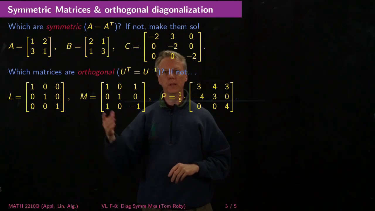
A matrix is orthogonally diagonalizable if and only if it is symmetric. math.la.t.mat.diagonalizable.orthogonally
Definition of matrix diagonalization math.la.d.mat.diagonalization
Eigenvectors of a symmetric matrix with different eigenvalues are orthogonal. math.la.t.mat.symmetric.eig.orthogonal
The spectral theorem for symmetric matrices math.la.t.mat.symmetric.spectral
- Created On
- August 21st, 2017
- 7 years ago
- Views
- 4
- Type
- Video
- Language
- English
- Content Type
- text/html; charset=utf-8
In this section we will back up and start simple. We begin with a definition of a totally general set of matrices, and see where that takes us.
Definition of symmetric matrix math.la.d.mat.symmetric
- License
- GFDL-1.2
- Submitted At
- September 11th, 2017
- 7 years ago
- Views
- 3
- Type
- Textbook
- Language
- English
- Content Type
- text/html